the test case in turn, and training with the 1 2 D ( h , h - PDF document

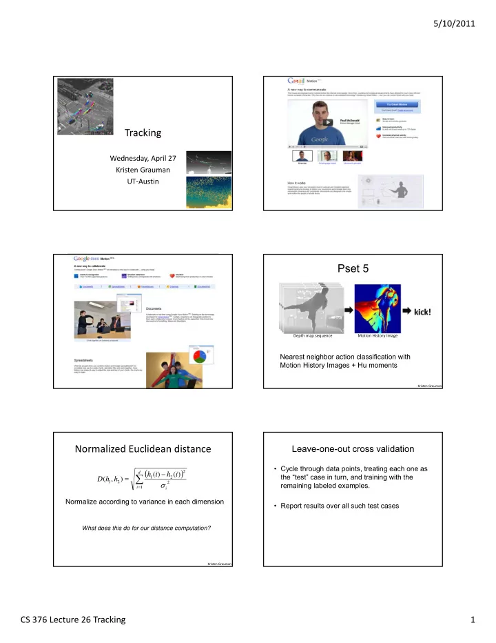
5/10/2011 Tracking Wednesday, April 27 Kristen Grauman UT ‐ Austin Pset 5 Depth map sequence Motion History Image Nearest neighbor action classification with Motion History Images + Hu moments Kristen Grauman Normalized Euclidean distance Leave-one-out cross validation • Cycle through data points, treating each one as    2 d h ( i ) h ( i )  the “test” case in turn, and training with the  1 2 D ( h , h ) 1 2  2 remaining labeled examples.  i 1 i Normalize according to variance in each dimension • Report results over all such test cases What does this do for our distance computation? Kristen Grauman CS 376 Lecture 26 Tracking 1

5/10/2011 Tracking: some applications Outline • Today: Tracking – Tracking as inference – Linear models of dynamics – Kalman filters Body pose tracking, Censusing a bat Video-based – General challenges in tracking activity recognition population interfaces Medical apps Surveillance Kristen Grauman Optical flow for tracking? Why is tracking challenging? If we have more than just a pair of frames, we could compute flow from one to the next: … … But flow only reliable for small motions, and we may have occlusions, textureless regions that yield bad estimates anyway… Motion estimation techniques Feature-based matching for motion • Direct methods Best matching • Directly recover image motion at each pixel from spatio-temporal Interesting point neighborhood image brightness variations Time t Time t+1 • Dense motion fields, but sensitive to appearance variations Search window • Suitable for video and when image motion is small • Feature-based methods • Extract visual features (corners, textured areas) and track them over multiple frames • Sparse motion fields, but more robust tracking • Suitable when image motion is large (10s of pixels) Search window is centered at the point where we last saw the feature, in image I1. Best match = position where we have the highest normalized cross-correlation value. Kristen Grauman CS 376 Lecture 26 Tracking 2

5/10/2011 Example: A Camera Mouse Example: A Camera Mouse Video interface: use feature tracking as mouse Specialized software for communication, games replacement • User clicks on the feature to be tracked • Take the 15x15 pixel square of the feature • In the next image do a search to find the 15x15 region with the highest correlation • Move the mouse pointer accordingly • Repeat in the background every 1/30th of a second James Gips and Margrit Betke http://www.bc.edu/schools/csom/eagleeyes/ James Gips and Margrit Betke http://www.bc.edu/schools/csom/eagleeyes/ Kristen Grauman Kristen Grauman A Camera Mouse Feature-based matching for motion Specialized software for communication, games • For a discrete matching search, what are the tradeoffs of the chosen search window size? • Which patches to track? • Select interest points – e.g. corners • Where should the search window be placed? • Near match at previous frame James Gips and Margrit Betke • More generally, taking into account the expected http://www.bc.edu/schools/csom/eagleeyes/ dynamics of the object Kristen Grauman Kristen Grauman Detection vs. tracking Detection vs. tracking … … t=1 t=2 t=20 t=21 Detection: We detect the object independently in each frame and can record its position over time, e.g., based on blob’s centroid or detection window coordinates Kristen Grauman Kristen Grauman CS 376 Lecture 26 Tracking 3

5/10/2011 Detection vs. tracking Detection vs. tracking … … Tracking with dynamics : We use image Tracking with dynamics : We use image measurements to estimate position of object, but measurements to estimate position of object, but also incorporate position predicted by dynamics, also incorporate position predicted by dynamics, i.e., our expectation of object’s motion pattern. i.e., our expectation of object’s motion pattern. Kristen Grauman Kristen Grauman Tracking with dynamics Tracking as inference • Use model of expected motion to predict where • The hidden state consists of the true parameters objects will occur in next frame, even before seeing we care about, denoted X . the image. • Intent : • The measurement is our noisy observation that results from the underlying state, denoted Y . – Do less work looking for the object, restrict the search. – Get improved estimates since measurement noise is tempered by smoothness, dynamics priors. • At each time step, state changes (from X t-1 to X t ) • Assumption : continuous motion patterns: and we get a new observation Y t . – Camera is not moving instantly to new viewpoint – Objects do not disappear and reappear in different places in the scene – Gradual change in pose between camera and scene Kristen Grauman Kristen Grauman Tracking as inference State vs. observation • The hidden state consists of the true parameters we care about, denoted X . • The measurement is our noisy observation that results from the underlying state, denoted Y . • At each time step, state changes (from X t-1 to X t ) and we get a new observation Y t . Hidden state : parameters of interest Measurement : what we get to directly observe • Our goal: recover most likely state X t given – All observations seen so far. – Knowledge about dynamics of state transitions. Kristen Grauman Kristen Grauman CS 376 Lecture 26 Tracking 4

5/10/2011 Tracking as inference: intuition Tracking as inference: intuition measurement Belief: prediction Belief: prediction Time t Time t+1 Corrected prediction Belief Measurement Corrected prediction old belief Time t Time t+1 Kristen Grauman Kristen Grauman Tracking as inference Independence assumptions • Prediction: • Only immediate past state influences current state – Given the measurements we have seen up to       P X X , , X P X X this point, what state should we predict?   t 0 t 1 t t 1   dynamics model  P X y , , y  t 0 t 1 • Measurement at time t depends on current state     • Correction:   P Y X , Y , X , Y , X P Y X   t 0 0 t 1 t 1 t t t – Now given the current measurement, what observation model state should we predict?   0  P X y , , y t t Kristen Grauman Kristen Grauman Questions Notation reminder x μ Σ ~ N ( , ) • How to represent the known dynamics that govern the changes in the states? • Random variable with Gaussian probability • How to represent relationship between state and distribution that has the mean vector μ and measurements, plus our uncertainty in the measurements? covariance matrix Σ . • How to compute each cycle of updates? • x and μ are d -dimensional, Σ is d x d . d =2 d =1 Representation : We’ll consider the class of linear If x is 1-d, we dynamic models, with associated Gaussian pdfs. just have one Σ parameter - Updates : via the Kalman filter.  the variance: σ 2 Kristen Grauman Kristen Grauman CS 376 Lecture 26 Tracking 5

5/10/2011 Example: randomly Linear dynamic model x Dx Σ ~ N ( ; )  drifting points t t 1 d • Describe the a priori knowledge about • Consider a stationary object, with state as position – System dynamics model: represents evolution • Position is constant, only motion due to random of state over time. noise term. x Dx Σ ~ N ( ; )  t t 1 d • State evolution is described by identity matrix D = I n x 1 n x n n x 1 – Measurement model: at every time step we get a noisy measurement of the state. y Mx Σ ~ N ( ; ) t t m m x 1 m x n n x 1 Kristen Grauman x Dx Σ Example: Constant Example: Constant ~ N ( ; )  t t 1 d y Mx Σ velocity (1D points) velocity (1D points) ~ N ( ; ) t t m • State vector: position p and velocity v 1 d position        p p ( t ) v p    t t 1 t 1 measurements t   1 d position x    t   v v v  t t t 1      1 t p      t 1 x D x noise     noise  t t t 1   0 1  v  states  t 1 • Measurement is position only   time p       t   y Mx noise 1 0 noise t t   v t Kristen Grauman Kristen Grauman Questions The Kalman filter • How to represent the known dynamics that govern the • Method for tracking linear dynamical models in changes in the states? Gaussian noise • How to represent relationship between state and • The predicted/corrected state distributions are measurements, plus our uncertainty in the measurements? Gaussian • How to compute each cycle of updates? – Only need to maintain the mean and covariance – The calculations are easy Representation : We’ll consider the class of linear dynamic models, with associated Gaussian pdfs. Updates : via the Kalman filter. Kristen Grauman Kristen Grauman CS 376 Lecture 26 Tracking 6