The Sunrise Integral and Elliptic Polylogarithms Luise Adams , - PowerPoint PPT Presentation

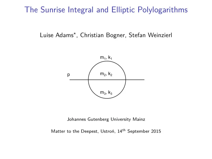
The Sunrise Integral and Elliptic Polylogarithms Luise Adams ⋆ , Christian Bogner, Stefan Weinzierl m 1 , k 1 m 2 , k 2 p m 3 , k 3 Johannes Gutenberg University Mainz n, 14 th September 2015 Matter to the Deepest, Ustro´

Short Introduction The Sunrise Integral in D = 2 The Sunrise Integral in D = 4 Elliptic Curves and Elliptic Integrals An elliptic curve can be written with the help of the Weierstrass equation: Y 2 Z + a 1 XYZ + a 3 YZ 2 = X 3 + a 2 X 2 Z + a 4 XZ 2 + a 6 Z 3 β and is topologically equivalent to a torus; 0 two integrals along the paths α, β are in the first λ α homology group of the torus ⇒ periods ω 1 , ω 2 1 elliptic integral = path integral along elliptic curve E ; ω 1 only well-defined mod Λ = { n 1 ω 1 + n 2 ω 2 : n 1 , n 2 ∈ Z } which defines a lattice ω 2 elliptic integrals E ( C ) − − − − − − − − → torus C \ Λ : elliptic integral gives an isomorphism from E ( C ) to C \ Λ 2 / 21

Short Introduction The Sunrise Integral in D = 2 The Sunrise Integral in D = 4 modified lattice Λ τ generated by 1 and τ = ω 2 /ω 1 : with q = e 2 π i τ Λ τ = Z τ + Z and it is Λ τ = Λ τ + k , k ∈ Z Under the exponential map J : C → C ∗ , z → e 2 π iz = w the lattice Λ τ in C is mapped to q Z in C ∗ → analytic isomorphism E τ = C / Λ τ → C ∗ / q Z The representation of the elliptic curve in C ∗ / q Z is called the Jacobi uniformization of the curve. Chain of mappings between the different representations of an elliptic curve Weierstrass Weierstrass normal ^ ^ z e 2 π iz Jacobi variable transformation periods ∫α dx/y, ∫β dx/y elliptic integrals Lattice Λ or Λτ ^ T orus z equation form y²=ax³+bx+c uniformization y β α ω 1 or 1 x ω 2 or τ 3 / 21

Short Introduction The Sunrise Integral in D = 2 The Sunrise Integral in D = 4 Classical and Elliptic Polylogarithms Multiple polylogarithms are special Z-sums with two different representations: x i 1 x i 2 x ik � 1) as nested sums: Li m 1 , m 2 ,..., m k ( x 1 , . . . , x k ) = . . . 1 2 k i m 1 i m 2 i mk 1 2 ∞≥ i 1 ≥ i 2 ≥···≥ i k ≥ 0 k 2) as iterated integrals: t k − 1 y t 1 dt 1 dt 2 dt k � � � With G ( z 1 , . . . , z k ; y ) = t 2 − z 2 . . . t k − z k and t 1 − z 1 0 0 0 k ! ( log y ) k we can define 1 G ( 0 , . . . , 0 ; y ) := G m 1 ,..., m k ( z 1 , . . . , z k ; y ) = G ( 0 , . . . , 0 , z 1 , . . . , z k − 1 , 0 , . . . , 0 , z k ; y ) and obtain � �� � � �� � m 1 − 1 m k − 1 � 1 � 1 1 Li m 1 , m 2 ,..., m k ( x 1 , x 2 , . . . , x k ) = ( − 1 ) k G m 1 , m 2 ,..., m k x 1 , x 1 x 2 , . . . , ( ⋆ ) x 1 x 2 . . . x k � y � z 1 , z 1 z 2 , . . . , z k − 1 ⇔ G m 1 , m 2 ,..., m k ( z 1 , z 2 , . . . , z k ; y ) = ( − 1 ) k Li m 1 , m 2 ,..., m k z k generalise eq. ( ⋆ ) (for P 1 \ { 0 , 1 , ∞} ) to a punctured elliptic curve E × � LHS: elliptic polylogarithms, RHS: iterated integrals on an elliptic curve 4 / 21

Short Introduction The Sunrise Integral in D = 2 The Sunrise Integral in D = 4 Elliptic polylogarithms ‘live’ on an elliptic curve; they are iterated integrals on the configuration space E ( n ) of an elliptic curve with n marked points [Brown, Levin 2013], [Levin, 1997] Basic idea: Average multivalued functions on a punctured elliptic curve E × = E \ { 0 } with respect to the multiplication by q arriving at � � q m 2 t 2 , q m 2 t 2 q m 1 t 1 q m 3 t 3 , . . . , q m r − 1 t r − 1 � , q m r t r u m 1 1 u m 2 . . . u m r r Li n 1 , n 2 ,..., n r � 2 q m r t r m 1 , m 2 ,..., m r ∈ Z The parameters u i dampen the singularities of the polylogs; Compute the pole structure in the u i coordinates, regularise the function with u i = exp ( 2 π i α i ) ⇒ the coefficients of the Taylor expansion around α i = 0 , i = 0 , 1 , . . . , r yield the multiple elliptic polylogarithms 5 / 21

II. The Sunrise Integral in D = 2 space-time dimensions m 1 , k 1 m 2 , k 2 p m 3 , k 3

Short Introduction The Sunrise Integral in D = 2 The Sunrise Integral in D = 4 The two-loop sunrise integral in D dimensions reads [Caffo, Czyz, Laporta, Remiddi 1998; Laporta, Remiddi 2004] : S ν 1 ν 2 ν 3 ( D , p 2 , m 1 , m 2 , m 3 ) = � � d D k 1 d D k 2 1 = ( µ 2 ) ν − D 2 ) ν 2 ( − ( p − k 1 − k 2 ) 2 + m 2 ( − k 2 1 + m 2 1 ) ν 1 ( − k 2 2 + m 2 D D 3 ) ν 3 i π i π 2 2 In its Feynman parameterisation the integral reads ( ν = ν 1 + ν 2 + ν 3 ) : � U ν − 3 2 D Γ( ν − D ) Γ( ν 1 )Γ( ν 2 )Γ( ν 3 )( µ 2 ) ν − D ω x ν 1 − 1 x ν 2 − 1 x ν 3 − 1 S ν 1 ν 2 ν 3 ( D , t ) = 1 2 3 F ν − D σ with the differential two-form ω = x 1 dx 2 ∧ dx 3 + x 2 dx 3 ∧ dx 1 + x 3 dx 1 ∧ dx 2 and the integration region σ = { [ x 1 : x 2 : x 3 ] ∈ P 2 | x i ≥ 0 , i = 1 , 2 , 3 } and the first and second graph polynomial ( t = p 2 ) U = x 1 x 2 + x 2 x 3 + x 1 x 3 , F = − x 1 x 2 x 3 t +( x 1 m 2 1 + x 2 m 2 2 + x 3 m 2 3 )( x 1 x 2 + x 2 x 3 + x 3 x 1 ) . 7 / 21

Short Introduction The Sunrise Integral in D = 2 The Sunrise Integral in D = 4 In D dimensions the integral S 111 satisfies a differential equation of order four:         P 4 d 4 dt 4 + P 3 d 3 dt 3 + P 2 d 2 dt 2 + P 1 d S 111 ( D , t ) = µ 2 [ c 12 T 12 + c 23 T 23 + c 13 T 13 ] dt + P 0     � �� �   =: L 4 ( D ) where the P i ’s and c ij ’s are polynomials in D , t and the masses and the T ij ’s are products of tadpoles [Adams, Bogner, Weinzierl, 2015] In D = 2 − 2 ǫ the integral S 111 and the differential operator L ( 0 ) can be 4 expanded in a Laurent series leading to a factorisable differential operator in ǫ 0 : 111 ( 2 , t ) = − 32 µ 2 t 2 ( 15 t 2 + 14 M 100 t + 77 ∆) L ( 0 ) 1 , a ( 2 ) L ( 0 ) 1 , b ( 2 ) L ( 0 ) 2 ( 2 ) S ( 0 ) � � p 2 ( t ) d 2 dt 2 + p 1 ( t ) d S ( 0 ) dt + p 0 ( t ) 111 ( 2 , t ) = p 3 ( t ) � [M¨ uller-Stach, Weinzierl, Zayadeh, 2013] L ( 0 ) 1 , a ( 2 ) L ( 0 ) 1 , b ( 2 ) L ( 0 ) 2 ( 2 ) S ( 1 ) in ǫ 1 : 111 ( 2 , t ) = I 1 ( t ) [later more] 8 / 21

Short Introduction The Sunrise Integral in D = 2 The Sunrise Integral in D = 4 First consider the equation F = 0 which defines together with the choice of an origin O an elliptic curve. x 3 Choose one of the σ P =(0:0:1) 3 intersection points of the integration region σ with the P =(0:1:0) variety defined by F = 0 as 2 x 2 origin, e.g. P 3 = [ 0 : 0 : 1 ] . P =(1:0:0) 1 x 1 Transform into Weierstrass normal form E : y 2 z = 4 x 3 − g 2 xz 2 − g 3 z 3 ˆ with O = [ 0 : 1 : 0 ] 9 / 21

Short Introduction The Sunrise Integral in D = 2 The Sunrise Integral in D = 4 Working with z = 1 one can factorise the RHS to y 2 = 4 ( x − e 1 )( x − e 2 )( x − e 3 ) with e 1 + e 2 + e 3 = 0 where the roots e i depend on t , the masses and the invariants g 2 = − 4 ( e 1 e 2 + e 2 e 3 + e 3 e 1 ) , g 3 = 4 e 1 e 2 e 3 With the assumption 0 ≤ m 1 ≤ m 2 ≤ m 3 it is e 2 ≤ e 3 < 0 < e 1 and one can find the periods of the elliptic curve in Weierstrass form: e 3 e 3 � � y = 4 µ 2 y = 4i µ 2 dx dx K ( k ′ ) Ψ 1 = 2 √ K ( k ) , Ψ 2 = 2 √ 4 4 D D e 2 e 1 where K ( x ) denotes the complete elliptic integral of the first kind 1 � dt K ( x ) = � ( 1 − t 2 )( 1 − x 2 t 2 ) 0 � with the (complementary) modulus k ( ′ ) : k = e 3 − e 2 e 1 − e 2 and √ � k ′ = 1 − k 2 = e 1 − e 3 e 1 − e 2 10 / 21

Short Introduction The Sunrise Integral in D = 2 The Sunrise Integral in D = 4 The periods Ψ 1 , Ψ 2 are the solutions of the homogeneous differential equation! [Adams, Bogner, Weinzierl (2013, 2014)] Consider the ratio of the two periods τ and the nome q : τ = i K ( k ′ ) q = e i πτ K ( k ) , and you can make a transformation of the variable t → q [Bloch, Vanhove, 2013] With variation of the constants one finds for a special inhomogeneous solution: q q 1 � � p 3 ( q ′′ )Ψ 1 ( q ′′ ) 3 S special = − µ 2 Ψ 1 ( q ) dq ′ dq ′′ π 2 p 2 ( q ′′ ) W ( q ′′ ) 2 q ′ q ′′ 0 0 d d with the Wronski determinant W = Ψ 1 dt Ψ 2 − Ψ 2 dt Ψ 1 11 / 21

Short Introduction The Sunrise Integral in D = 2 The Sunrise Integral in D = 4 Aim: Express the special solution in terms of the homogeneous solutions and generalised (elliptic) polylogarithms Consider the elliptic curve E i defined by F = 0 with origin P i → transform into Weierstrass normal form ˆ E with origin Q i , i = [ 0 : 1 : 0 ] → Periods Ψ 1 , Ψ 2 of ˆ E define a lattice Λ → map from ˆ E to the torus C / Λ with the elliptic integral ∞ � z = 1 dx [ x : y : 1 ] → ˆ � Ψ 1 4 ( x − e 1 )( x − e 2 )( x − e 3 ) x 12 / 21

Short Introduction The Sunrise Integral in D = 2 The Sunrise Integral in D = 4 � e 1 − e 2 z i = 1 F ( u i , k ) → intersection points Q j , k → ˆ with u i = ((i,j,k) 2 K ( k ) x j , k − e 2 as cyclic permutation of (1,2,3) and F ( z , x ) as the incomplete elliptic integral of the first kind z � dt F ( z , x ) = � ( 1 − t 2 )( 1 − x 2 t 2 ) 0 ( Q i , j → [ x i , j : y i , j : 1 ] is the image of the point P i ∈ E j on ˆ E ) → map to the Jacobi uniformization C ∗ / q 2 Z with z → w = e 2 π i ˆ z ˆ � � i π F ( u i , k ) → points ˆ z i → w i with w i = exp K ( k ) 13 / 21