The reasons behind some classical constructions in analysis V. - - PowerPoint PPT Presentation

the reasons behind some classical constructions in
SMART_READER_LITE
LIVE PREVIEW

The reasons behind some classical constructions in analysis V. - - PowerPoint PPT Presentation

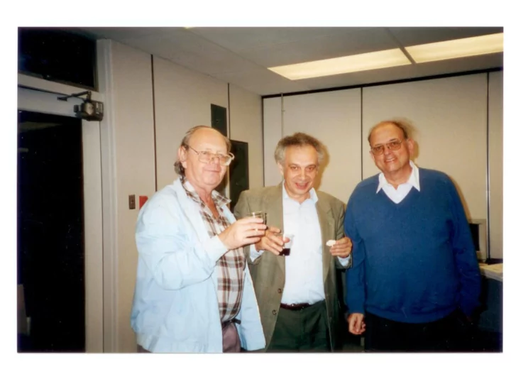
The reasons behind some classical constructions in analysis V. Milman Tel-Aviv University In the memory of a great scientist and a good friend, Aleksander (Olek) Peczyski June 2014, Bdlewo, Poland 2/25 Instead of an Introduction: some


slide-1
SLIDE 1
slide-2
SLIDE 2

2/25

The reasons behind some classical constructions in analysis

  • V. Milman

Tel-Aviv University

In the memory of a great scientist and a good friend, Aleksander (Olek) Pełczyński June 2014, Będlewo, Poland

slide-3
SLIDE 3

3/25

Instead of an Introduction: some geometric results

What should we call “duality”? Consider the class Cvx (Rn) of all lower-semi-continuous convex functions f : Rn → R ∪ {+∞}. The Legendre transform is the map Lϕ(x) = sup

y∈Rn

x, y − ϕ(y)

  • .

Of course, there are many “Legendre transforms”: We may select 0

  • f the space, a scalar product and a shift for a function.

Theorem (Artstein–Milman)

  • 1. Assume T : Cvx (Rn) → Cvx (Rn) satisfies:

(a) T · T ϕ = ϕ (for any ϕ ∈ Cvx (Rn)); (b) ϕ ≤ ψ implies T ϕ ≥ Tψ.

Then T is a Legendre transform. It means that Cvx (Rn) has a unique duality structure!

slide-4
SLIDE 4

4/25

Let us embed K(Rn) = {K ⊆ Rn | closed convex} into Cvx (Rn) by “convex characteristic” functions: K − → 1∞

K =

  • x ∈ K,

+∞ x ∈ K. For K ∈ K0(Rn) = {K ∈ K (Rn) | 0 ∈ K}, define its gauge function (or Minkowski functional M (1∞

K )) – 1-homogeneous

convex function xK, “generalized” norm, s.t. K = {x ∈ Rn | xK ≤ 1}. Let H0 = {xK | K ∈ K0(Rn)}. Define the Minkowski map M(1∞

K ) = xK ∈ H0

and the support map S(1∞

K ) = sup{x, y | y ∈ K} ∈ H0.

Obviously, M : K0(Rn) → H0 is an order preserving map (1-1 and

  • nto) and S : K0(Rn) → H0 is an order reversing map.
slide-5
SLIDE 5

5/25

We continue the theorem:

Theorem (Artstein–Milman)

  • 2. There is a unique order reversing extension of the support

map S to Cvx (Rn) which is the Legendre transform. And what is the polarity map on K0 (Rn) K → K ◦ = {x ∈ Rn | x, y ≤ 1 ∀y ∈ K}? K ◦is defined if 0 ∈ K. So, let Cvx0 (Rn) = {f ∈ Cvx (Rn) | f (x) ≥ 0 and f (0) = 0} be the class of geometric convex functions.

  • 3. There is a unique order reversing extension of the polarity

map {1∞

K → 1∞ K ◦ | K ∈ K0} to Cvx0 (Rn) \0 defined by

Af = sup x, y − 1 f (y) , and A(0) := 1∞

{0}. (By extension we mean that A1∞ K = 1∞ K ◦)

slide-6
SLIDE 6

6/25

There are ONLY two dualities on Cvx0 (Rn) – L and A:

Theorem (Artstein–Milman)

Let n ≥ 2. The maps L and A are (essentially) the only order reversing involutions on Cvx0(Rn). Precisely: if T : Cvx0 → Cvx0 is

  • 1. involution T · T = Id.
  • 2. order reversing: ∀f , g ∈ Cvx0 we have f ≤ g ⇒ Tf ≥ Tg,

then ∃C > 0 and B ∈ GLn, symmetric, s.t. either ∀f ∈ Cvx0, Tf = L(f (Bx))

  • r

∀f ∈ Cvx0, Tf = CA(f (Bx)). (when n = 1 there are 8 such different dualities)

slide-7
SLIDE 7

7/25

Consider the order preserving map (involution) J = LA = AL which connects two dualities (supporting map – Legendre transform L, and geometric dualityA). J is a very interesting map Cvx0 → Cvx0, order preserving. It is the gauge map: [Fact]Artstein-Milman. J is the only order preserving extension of the Minkowski map M onto Cvx0(Rn), i.e. J (1∞

K ) ≡ M(1∞ K ) = xK.

So, on the class of convex functions we have the notion of support function, Minkowski functional and polarity!

slide-8
SLIDE 8

8/25

Classical constructions in analysis which appear (uniquely) from elementary (simplest) properties

Now let us look into the continuation of the previous geometric ideas applied to the problems of Analysis. We start with a characterization of the classical Fourier transform F on Rn : Ff = e−2πix,yf (y)dy. Let S be the Schwartz class

  • f “rapidly” decreasing (infinitely smooth) functions on Rn.

Theorem (Artstein, Faifman, Milman)

Assume we are given a bijective transform F : S → S, s.t. ∀f , g ∈ S we have F(f · g) = Ff ∗ Fg. Then ∃ diffeomorphism ω : Rn → Rn s.t. either ∀f ∈ S, Ff = F(f ◦ ω)

  • r ∀f ∈ S, Ff = F(f ◦ ω).
slide-9
SLIDE 9

9/25

Real linearity and continuity of F is the automatic consequence. Previous versions contained more conditions and were proved jointly with S. Alesker. Joining these results with the previous theorem we may state that if F : S → S s.t. ∀f , g ∈ S F(f · g) = Ff ∗ Fg, F(f ∗ g) = Ff · Fg, then ∃ linear A ∈ GLn, |det(A)| = 1, s.t. either ∀f ∈ S, Ff = F(f ◦ A)

  • r

∀f ∈ S, Ff = F(f ◦ A).

slide-10
SLIDE 10

10/25

Derivative; Approach through the chain rule

What algebraic property characterizes derivative on R? Let C1

b(R) =

  • f ∈ C1(R) |

f bounded from above or from below (or both)

  • .

write (f ◦ g)(x) := f (g(x)) (composition). We say, T : Dom(T) = C1(R) → Im(T) ⊂ C(R) is non-degenerate if ∃x0 ∈ R, h0 ∈ C1(R), (Th0)(x0) = 0, (1) ∃x2 ∈ R, h2 ∈ C1

b(R), (Th2)(x2) < 0.

(2) (a very weak surjectivity type condition).

slide-11
SLIDE 11

11/25

Theorem (Artstein, König, Milman)

Let T : Dom(T) := C1(R) → Im(T) ⊂ C(R) be an operation satisfying the chain rule T(f ◦ g) = (Tf ) ◦ g · Tg; f , g ∈ D(T). (3) Assume that T is non-degenerate in the sense of (1)+(2). (Normalizing conditions) T(2Id) = 2 (is a constant function), then Tf = f ′ is the only solution. No linearity or any kind of continuity of T is assumed, but is the consequence (under the above conditions) of the chain rule only.

slide-12
SLIDE 12

12/25

Without the normalization condition the result is: ∃ strictly monotone continuously differentiable function G(x) and p > 0, s.t. Tf =

  • d(G ◦ f )

dG

  • p

· sgn(f ′). Note: If T(f ◦ g) = Tf · Tg (T : Ck → C) (and not degenerate at any x ∈ R) then Tf = 1, ∀f ∈ Ck. So, we need (Tf ) ◦ g · Tg to build a non-degenerate operation. The same answer may be written differently: ∃H ∈ C (R), H > 0 and p > 0 s.t. Tf = H(f (x)) H(x) ·

  • f ′

p sgn(f ′).

slide-13
SLIDE 13

13/25

The chain rule (3) has a natural (and unique) domain on which it acts (with the image inside C(R)), and it is C1(R). Facts from (A-K-M). Let T : L → C(R) satisfy (3) for f , g, f ◦ g ∈ L. If:

◮ L = C(R) and ∃g0 ∈ C and x0 ∈ R s.t. (Tg0)(x0) = 0.Then

T|Cb(R) ≡ 0.

◮ C ∞(R) ⊂ L ⊂ C1(R) =

⇒ T maybe extended to C1(R); So the natural Dom(T) is C1!

slide-14
SLIDE 14

14/25

Rigidity of the chain rule

To what extent is the standard chain rule inferred by a much weaker version? Let V : C1(R) → C(R) be non-degenerate, i.e.

  • 1. For any x ∈ R there is f ∈ C1(R) such that Vf (x) = 0, and
  • 2. For any x ∈ R there are y ∈ R and f ∈ C1(R) such that

f (y) = x and Vf (y) = 0.

slide-15
SLIDE 15

15/25

Theorem (König-Milman)

Assume that V , T1,T2 : C1(R) → C(R) are operators such that the equation V (f ◦ g) = (T1f ) ◦ g · (T2g) holds for all f , g ∈ C1(R). Assume that V is non-degenerate. There is a solution T of the chain rule equation T(f ◦ g) = (Tf ) ◦ g · Tg, s.t. (Vf )(x) = c1(f (x))c2(x) · (Tf )(x) (T1f )(x) = c1(f (x)) · (Tf )(x) (T2f )(x) = c2(x) · (Tf )(x), i.e. all three a priori different operators are essentially the same (a strong super rigidity).

slide-16
SLIDE 16

16/25

Stability of the Chain Rule

T : C1(R) → C(R) is locally non-degenerate if ∀ open interval J ⊂ R, ∀x ∈ J, ∃g ∈ C1(R), y ∈ R, s.t. g(y) = x, Im(g) ⊂ J and Tg(y) = 0.

Theorem (König-Milman)

Fix T : C1(R) → C(R) and B : R3 → R such that ∀f , g ∈ C1 and ∀x ∈ R T(f ◦ g)(x) = Tf ◦ g(x) · Tg(x) + B(x, f ◦ g(x), g(x)). Assume that T is locally non-degenerate and Tf depends non-trivially on f ′. Then B = 0 (and T satisfies the chain rule).

slide-17
SLIDE 17

17/25

Even more rigidity

Consider the “chain rule inequality” T (f ◦ g) ≤ (Tf ) ◦ g · Tg (∗) for T : C1 (R) → C(R), Dom(T) = C1(R). Assume that T satisfies the following:

◮ non-degeneration: ∀ open interval I ⊂ R, ∀x ∈ I,

∃g ∈ C1(R) s.t. g(x) = x, Im(g) ⊂ I and Tg(x) > 1.

◮ T is pointwise continuous: ∀f , fn ∈ C1(R) s.t fn → f ,

f ′

n → f ′ uniformly on compact subsets we have

(Tfn) (x) → (Tf ) (x) pointwise for all x ∈ R.

slide-18
SLIDE 18

18/25

Theorem (König-Milman)

For T as above assume also ∃x ∈ R s.t T(−Id)(x) < 0. Then ∃H ∈ C(R), H > 0, ∃p > 0 and A ≥ 1 s.t Tf =

  • H◦f

H |f ′|p

for f ′ ≥ 0 −AH◦f

H |f ′|p

for f ′ < 0. Note:

◮ For A = 1, T satisfies the chain rule equation: we have

equality in (∗).

◮ For both f and g non-decreasing we automatically have

equality in (∗).

◮ Actually, the same is true if for some C > 0

T (f ◦ g) ≤ C · (Tf ) ◦ g · Tg and even much more generally (the answer is slightly modified).

slide-19
SLIDE 19

19/25

The following classically sound functional statement is used: We say that K : R → R is submultiplicative if K(αβ) ≤ K(α)K (β) , ∀α, β ∈ R.

Theorem (König-Milman)

Let K be submultiplicative, measurable and continuous at 0 and at

  • 1. Assume K(−1) < 0 < K(1). Then ∃p > 0 s.t.

K(α) =

  • αp

for α ≥ 0 −A |α|p for α < 0 (and K(−1) = −A ≤ −1). [every assumption in the theorem is needed] As a corollary, K must be multiplicative on R+.

slide-20
SLIDE 20

20/25

Approach through Leibniz rule

Theorem (König-Milman)

Suppose T : C1(R) → C(R) satisfies the Leibniz product formula T(f · g) = Tf · g + f · Tg; f , g ∈ C1(R). Then there are continuous functions c(x), d(x) such that Tf (x) = c(x)f ′(x) + d(x)f (x) ln |f (x)|, f ∈ C1(R), x ∈ R. (If T also maps C2(R) into C1(R), then Tf = cf ′.) We see that there exist (only!) two domains on which Leibniz’s rule acts:

  • 1. C(R) with the only solution being the entropy function

(Goldmann-Šemrl);

  • 2. C1(R) with 2 solutions, f ′ and f · ln |f |, and their linear

combination.

slide-21
SLIDE 21

21/25

Remark: Suppose T : C1(R) → C(R) satisfies the Leibniz rule and the chain rule operator equations T(f · g) = Tf · g + f · Tg, T(f ◦ g) = (Tf ) ◦ g · Tg, for all f , g ∈ C1(R). Then T is either identically 0 or the derivative, Tf = f ′. However: Let C(R>1)+ := {f ∈ C(R>1)| f > 1} and H(x) := x ln |x|. Then the operation T defined by Tf (x) := H(f (x))/H(x) yields a map T : C(R>1)+ → C(R) satisfying the Leibniz rule and the chain rule functional equations which is different from the derivative on the subset of positive C1(R>1) functions.

slide-22
SLIDE 22

22/25

We know a description of all solutions T and Ai of T(f · g) = Tf · A1g + Tg · A2f and there are just three more families of such solutions! And only

  • ne of them is non-degenerate. Moreover, we again observe

“super-rigidity” of a “Leibniz rule” structure.

slide-23
SLIDE 23

23/25

Theorem (König-Milman)

Let V , T1, T2 : C1(R) → C(R) be operators such that V (f · g) = (T1f ) · g + f · (T2g) (4) is satisfied for all f , g ∈ C1(R). Then there are continuous functions a, b, c1,c2 ∈ C(R) such that with (Tf )(x) := b(x)f ′(x) + a(x)f (x) ln |f (x)| we have (Vf )(x) = (Tf )(x) + (c1(x) + c2(x))f (x) (T1f )(x) = (Tf )(x) + c1(x)f (x) (T2f )(x) = (Tf )(x) + c2(x)f (x). The formula for (Tf )(x) represents the general solution of (4) in the case when V = T1 = T2 = T.

slide-24
SLIDE 24

24/25

It is surprising how rigid are simple relations which define (almost uniquely) basic operations/constructions in geometry and analysis. One more example:

Theorem (König-Milman)

Let k ∈ N, T : Ck(R) → C(R) be an operator and B : R × Rk × Rk → R be a function such that T(f · g)(x) = Tf (x) · g(x) + f (x) · Tg(x)+ B(x, f (x), . . . , f (k−1(x), g(x), . . . g(k−1)(x)) holds for all f , g ∈ Ck(R) and x ∈ R. Let T annihilate all polynomials of order ≤ k − 1. Then Tf = d · f (k) for d ∈ C(R), and B has the form B(x, f (x), . . . , g(k−1)(x)) = d(x)

k−1

j=1

k j

  • f (j)(x)g(k−j)(x).
slide-25
SLIDE 25

25/25

And the Laplacian case

Theorem (König-Milman)

Let n ∈ N. Let T : C2(Rn, R) → C(Rn, R) be an operator and B be a function B : Rn × R × Rn × R × Rn → R s.t. T(f · g)(x) = Tf (x) · g(x) + f (x) · Tg(x) + B(x, f (x), f ′(x), g(x), g′(x) holds for all f , g ∈ C2(Rn, R) and all x ∈ Rn. Let T annihilate all affine functions and be orthogonally invariant, i.e. T(f ◦ ϕ) = (Tf ) ◦ ϕ for all ϕ ∈ O(n). Then T is a multiple of the Laplacian: there is d ∈ C(R≥0, R) such that Tf (x) = d(||x||)∆f (x), B(x, f (x), f ′(x), g(x), g′(x)) = d(||x||)f ′(x), g′(x). holds for all f , g ∈ C2(Rn, R),x ∈ Rn, and ||x|| is Euclidean norm.