
SLIDE 1
The Quantum Program in One Dimension - So Far
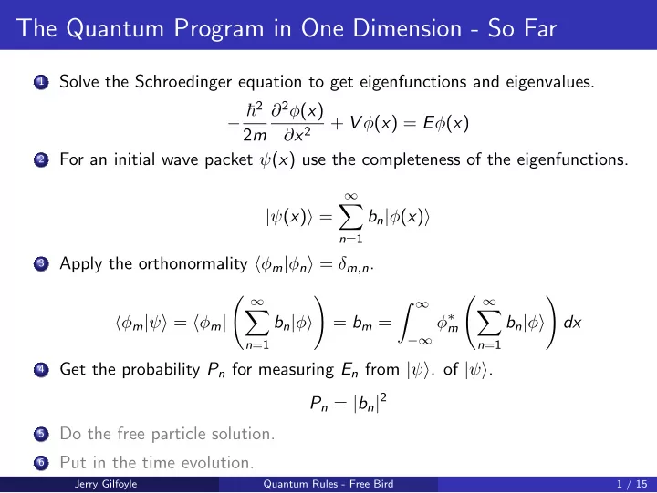
1
Solve the Schroedinger equation to get eigenfunctions and eigenvalues. − 2 2m ∂2φ(x) ∂x2 + V φ(x) = Eφ(x)
2
For an initial wave packet ψ(x) use the completeness of the eigenfunctions. |ψ(x) =
∞
- n=1
bn|φ(x)
3
Apply the orthonormality φm|φn = δm,n. φm|ψ = φm| ∞
- n=1
bn|φ
- = bm =
∞
−∞
φ∗
m
∞
- n=1
bn|φ
- dx
4
Get the probability Pn for measuring En from |ψ. of |ψ. Pn = |bn|2
5
Do the free particle solution.
6
Put in the time evolution.
Jerry Gilfoyle Quantum Rules - Free Bird 1 / 15