The Problem of Temporal Abstraction How do we connect the high level - - PowerPoint PPT Presentation

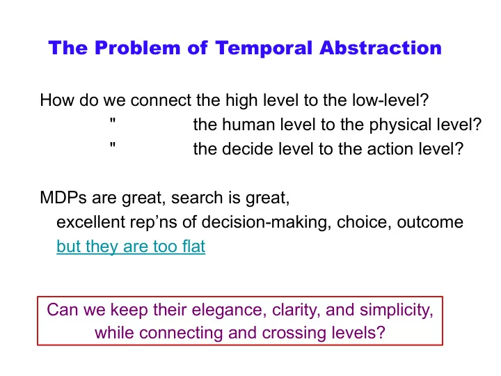
The Problem of Temporal Abstraction

How do we connect the high level to the low-level? " the human level to the physical level? " the decide level to the action level? MDPs are great, search is great, excellent rep’ns of decision-making, choice, outcome but they are too flat Can we keep their elegance, clarity, and simplicity, while connecting and crossing levels?

Goal: Extend RL framework 
 to temporally abstract action

• While minimizing changes to

❖ Value functions ❖ Bellman equations ❖ Models of the environment ❖ Planning methods ❖ Learning algorithms

• While maximizing generality

❖ General dynamics and rewards ❖ Ability to express all courses of behavior ❖ Minimal commitments to other choices

• Execution, e.g., hierarchy, interruption, intermixing with

planning

• Planning, e.g., incremental, synchronous, trajectory

based, “utility” problems

• State abstraction and function approximation
• Creation/Constructivism

It’s a dimensional thing

Options – Temporally Abstract Actions

E.g., the docking option:

: hand-crafted controller

: terminate when docked or charger not visible

Execution is nominally hierarchical (call-and-return) An option is a triple,

is the policy followed during o is the probability of the option continuing (not terminating) in each state

...there are also “semi-Markov” options

• = hπo, γoi

πo : S × A → [0, 1] γo : S → [0, γ] πo γo

Options are like actions

Just as a state has a set of actions, It also has a set of options, Just as we can have a flat policy, over actions, We can have a hierarchical policy, over options, To execute h in s : select option o with probability follow o until it terminates, in s’ then choose a next option with probability again, and so on Every hierarchical policy determines a flat policy Even if all the options are Markov, f (h) is usually not Markov Actions are a special case of options

A(s) O(s) π : S × A → [0, 1] π = f(h) h : O × S → [0, 1]

h(o|s) h(o0|s0)

Value Functions with Temporal Abstraction

A new set of optimization problems

Now consider a limited set of options and hierarchical policies that choose only from them

O

Define value functions for hierarchical policies and options: vO

∗ (s) = max h∈Π(O) vh(s)

qO

∗ (s, o) = max h∈Π(O) qh(s, o)

h ∈ Π(O) vh(s) = E ⇥ Rt+1 + γRt+2 + γ2Rt+3 + · · ·

• St = s, At:∞ ∼ h

⇤ qh(s, o) = E[Gt | St = s, At:t+k−1 ∼ πo, k ∼ γo, At+k:∞ ∼ h]

Options define a
 Semi-Markov Decision Process (SMDP)

• verlaid on the MDP

Discrete time Homogeneous discount Continuous time Discrete events Interval-dependent discount Discrete time Overlaid discrete events Interval-dependent discount

A discrete-time SMDP overlaid on an MDP. Can be analyzed at either level.

MDP SMDP Options

• ver MDP

State Time

Models of the Environment with Temporal Abstraction

Planning requires models of the consequences of action The model of an action has a reward part and a state transition part: As does the model of an option:

r(s, a) = E[Rt+1 | St = s, At = a] p(s0|s, a) = Pr{St+1 = s0 | St = s, At = a} r(s, o) = E ⇥ Rt+1 + · · · + γk−1Rt+k

• St = s, At:t+k−1 ∼ πo, k ∼ γo

⇤

p(s0|s, o) =

1

X

k=1

Pr{St+k = s0, termination at t + k | St = s, At:t+k1 ∼ πo} γk

Bellman Equations with Temporal Abstraction

For policy-specific value functions:

vh(s) = X

• h(o|s)

" r(s, o) + X

s0

p(s0|s, o)vh(s0) # vh qh(s, o) = r(s, o) + X

s0

p(s0|s, o) X

h(o0|s0)qh(s0, o0)

r(s, o) s0 s, o a0

h

p

qh

s s0

• r(s, o)

p

h

Planning with Temporal Abstraction

Reduces to conventional value iteration if

Initialize: Iterate: V (s) ← 0, ∀s ∈ S V (s) ← max

• "

r(s, o) + X

s0

p(s0|s, o)V (s0) # V → vO

∗

hO

⇤ (s) = greedy(s, vO ⇤ ) = arg max

• 2O

" r(s, o) + X

s0

p(s0|s, o)vO

⇤ (s0)

# O = A

Rooms Example

• 2

HALLWAYS

• 1

8 multi-step options

up down right left (to each room's 2 hallways)

G2 4 stochastic primitive actions

Fail 33%

• f the time

G1

Target Hallway

Policy of

• ne option:

Sutton, Precup, & Singh, 1999

γ = .9

All rewards zero, except +1 into goal

Planning is much faster with Temporal Abstraction

Iteration #0 Iteration #1 Iteration #2 with with ce cell-to to-ce cell primitive primitive actions actions Iteration #0 Iteration #1 Iteration #2 with with room-to-room room-to-room

• ption
• ptions

V(goal)=1 V(goal)=1

Without TA With TA

Temporal Abstraction helps even with Goal≠Subgoal
 given both primitive actions and options

Iteration #1 Initial values Iteration #2 Iteration #3 Iteration #4 Iteration #5

Iteration #1 Initial values Iteration #2 Iteration #3 Iteration #4 Iteration #5

why?

Temporal Abstraction helps even with Goal≠Subgoal
 given both primitive actions and options

Temporal abstraction also speeds learning about path-to-goal

SMDP Theory Provides a lot of this

• Policies over options: µ : S × O a [0,1]
• Value functions over options: V

µ(s), Q µ (s,o), V O *(s), QO * (s,o)

• Learning methods: Bradtke & Duff (1995), Parr (1998)
• Models of options
• Planning methods: e.g. value iteration, policy iteration, Dyna...
• A coherent theory of learning and planning with courses of

action at variable time scales, yet at the same level But not all. The most interesting issues are beyond SMDPs...

Hierarchical policies over options: h(o|s)

vh(s), qh(s, o), vO

∗ (s), qO ∗ (s, o)

: r(s, o), p(s0|s, o)

Outline

• The RL (MDP) framework
• The extension to temporally abstract “options”

❖ Options and Semi-MDPs ❖ Hierarchical planning and learning

• Rooms example
• Between MDPs and Semi-MDPs

❖ Improvement by interruption (including Spy plane demo) ❖ A taste of

• Intra-option learning
• Subgoals for learning options
• RoboCup soccer demo

Interruption

Idea: We can do better by sometimes interrupting ongoing options

• forcing them to terminate before says to

Theorem: For any hierarchical policy suppose we interrupt its options one or more times, t, when the action we are about to take o, is such that

γo h : O × S → [0, 1],

qh(St, o) < qh(St, h(St))

to obtain h’, Then h’ ≥ h (it attains more or equal reward everywhere) Application: Suppose we have determined and thus Then h’ is guaranteed better than and is available with no further computation

qO

∗

h = hO

∗

hO

∗

range (input set) of each run-to-landmark controller landmarks

S G

Landmarks Task

Task: navigate from S to G as fast as possible 4 primitive actions, for taking tiny steps up, down, left, right 7 controllers for going straight to each one of the landmarks, from within a circular region where the landmark is visible In this task, planning at the level of primitive actions is computationally intractable, we need the controllers

S G

SMDP Solution (600 Steps) Termination-Improved Solution (474 Steps)

Termination Improvement for Landmarks Task

Allowing early termination based on models improves the value function at no additional cost!

Spy Plane Example

• Mission: Fly over (observe) most

valuable sites and return to base

• Stochastic weather affects
• bservability (cloudy or clear) of sites
• Limited fuel
• Intractable with classical optimal

control methods

• Temporal scales:

❖ Actions: which direction to fly now ❖ Options: which site to head for

• Options compress space and time

❖ Reduce steps from ~600 to ~6 ❖ Reduce states from ~1010 to ~106

10 50 50 50 100 25 15 (reward) 5 25 8

Base

100 decision steps

• ptions

(mean time between weather changes)

any state ~1010 sites only ~106

qO

⇤ (s, o) = r(s, o) +

X

s0

p(s0|s, o)vO

⇤ (s0)

Spy Drone

30 40 50 60 TI SMDP Static

Spy Plane Example (Results)

• SMDP planner:

❖ Assumes options followed to

completion

❖ Plans optimal SMDP solution

• SMDP planner with interruption

❖ Plans as if options must be

followed to completion

❖ But actually takes them for only

• ne step

❖ Re-picks a new option on every

step

• Static planner:

❖ Assumes weather will not change ❖ Plans optimal tour among clear

sites

❖ Re-plans whenever weather

changes Low Fuel High Fuel

Expected Reward/Mission

Temporal abstraction finds better approximation than static planner, with little more computation than SMDP planner

SMDP Planner Static Re-planner SMDP 
 planner 
 with 
 interruption

Outline

• The RL (MDP) framework
• The extension to temporally abstract “options”

❖ Options and Semi-MDPs ❖ Hierarchical planning and learning

• Rooms example
• Between MDPs and Semi-MDPs

❖ Improvement by interruption (including Spy plane demo) ❖ A taste of

• Intra-option learning
• Subgoals for learning options
• RoboCup soccer demo

Intra-Option Learning Methods 
 for Markov Options

Proven to converge to correct values, under same assumptions as 1-step Q-learning

Idea: take advantage of each fragment of experience

SMDP Q-learning:

• execute option to termination, keeping track of reward along

the way

• at the end, update only the option taken, based on reward and

value of state in which option terminates Intra-option Q-learning:

• after each primitive action, update all the options that could have

taken that action, based on the reward and the expected value from the next state on

Intra-Option Learning Methods 
 for Markov Options

Proven to converge to correct values, under same assumptions as 1-step Q-learning Idea: take advantage of each fragment of experience Intra-Option Learning: after each primitive action, update all the options that could have taken that action SMDP Learning: execute option to termination,then update only the

• ption taken

Returning to the rooms example…

• 2

HALLWAYS

• 1

8 multi-step options

up down right left (to each room's 2 hallways)

G2 4 stochastic primitive actions

Fail 33%

• f the time

G1

Target Hallway

Policy of

• ne option:

Sutton, Precup, & Singh, 1999

γ = .9

All rewards zero, except +1 into goal

Intra-Option Value Learning
 in the Rooms Example

Intra-option methods learn correct values without ever

taking the options! SMDP methods are not applicable here

Random start, goal in right hallway, random actions

• 4
• 3
• 2
• 1

1000 1000 6000 2000 3000 4000 5000 6000

Episodes Episodes

Option values Average value of greedy policy

Learned value Learned value Upper hallway

• ption

Left hallway

• ption

True value True value

• 4
• 3
• 2

1 10 100

Value of Optimal Policy

Intra-Option Model Learning

Intra-option methods work much faster than SMDP methods

Random start state, no goal, pick randomly among all options

Options executed

State prediction error

0.1 0.2 0.3 0.4 0.5 0.6 0.7 20,000 40,000 60,000 80,000 100,000

SMDP SMDP Intra Intra SMDP 1/t

Max error Avg. error

SMDP 1/t

1 2 3 4 20,000 40,000 60,000 80,000 100,000

Options executed

SMDP Intra SMDP 1/t SMDP Intra SMDP 1/t

Reward prediction error

Max error

• Avg. error

Options Depend on Outcome Values

Large Outcome Values Small Outcome Values Learned Policy: Avoids Negative Rewards Learned Policy: Shortest Paths Small negative rewards on each step g = 10 g = 1 g = 0 g = 0

Summary: Benefits of Options

• Transfer of knowledge

❖ Solutions to sub-tasks can be saved and reused ❖ Domain knowledge can be provided as options and subgoals

• Potentially much faster learning and planning

❖ By representing action at an appropriate temporal scale

• Models of options are a form of knowledge representation

❖ Expressive ❖ Clear ❖ Suitable for learning and planning

• Much more to learn than just one policy, one set of values

❖ A framework for “constructivism” or “continual learning” – for

finding models of the world that are useful for rapid planning and learning

Conclusions

• We have come a long way toward linking human-level choices to

microscopic actions

❖ Temporally abstract facts, and estimates of them - knowledge! ❖ A theory of how to combine known subcontrollers (behaviors) ❖ Beginnings of how to learn them efficiently and without interference

• Resolution of the “subgoal credit-assignment” problem
• We have shown how the high-level can mirror the low

❖ It’s all choices, states, and values ❖ A minimal extension of existing RL/MDP ideas

• The state assumption remains a problem

❖ Someday options may revolutionize our notion of state and of

perception