
SLIDE 1
INSTITUTE OF NEUROSCIENCE AND MEDICINE (INM-1)
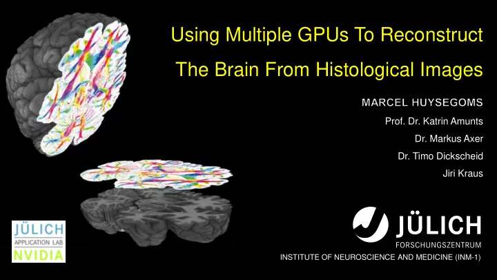
Using Multiple GPUs To Reconstruct The Brain From Histological Images
- Prof. Dr. Katrin Amunts
- Dr. Markus Axer
- Dr. Timo Dickscheid
Jiri Kraus