the 60 th cors annual conference decomposition based
play

The 60 th CORS Annual Conference Decomposition-Based Exact - PowerPoint PPT Presentation

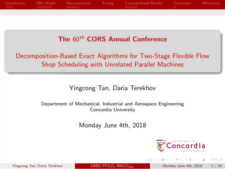
Introduction MIP Model Decomposition Tuning Computational Results Conclusion References The 60 th CORS Annual Conference Decomposition-Based Exact Algorithms for Two-Stage Flexible Flow Shop Scheduling with Unrelated Parallel Machines


  1. Introduction MIP Model Decomposition Tuning Computational Results Conclusion References The 60 th CORS Annual Conference Decomposition-Based Exact Algorithms for Two-Stage Flexible Flow Shop Scheduling with Unrelated Parallel Machines Yingcong Tan, Daria Terekhov Department of Mechanical, Industrial and Aerospace Engineering Concordia University Monday June 4th, 2018 Yingcong Tan, Daria Terekhov LBBD FF 2 | (1 , RM ) | C max Monday June 4th, 2018 1 / 26

  2. Introduction MIP Model Decomposition Tuning Computational Results Conclusion References Agenda 1 Introduction 2 MIP Model 3 Decomposition 4 Tuning 5 Computational Results 6 Conclusion Yingcong Tan, Daria Terekhov LBBD FF 2 | (1 , RM ) | C max Monday June 4th, 2018 2 / 26

  3. Introduction MIP Model Decomposition Tuning Computational Results Conclusion References Problem Definition Flexible Flow Shop Scheduling Problem Flow Shop: Given a set of jobs to be processed on a set of stages following the same route . Flexible: Each stage can have a single or multiple parallel machines 1 Identical : p 1 = p 2 2 Uniform : p 1 = α ∗ p 2 where α is machine-speed factor 3 Unrelated : p 1 � = p 2 Goal: Find the optimal job schedule with respect to a certain objective value Yingcong Tan, Daria Terekhov LBBD FF 2 | (1 , RM ) | C max Monday June 4th, 2018 3 / 26

  4. Introduction MIP Model Decomposition Tuning Computational Results Conclusion References Example of Two-Stage Flexible Flow Shop Figure: Two Stages Manufacturing System. (Lin and Liao 2003) Yingcong Tan, Daria Terekhov LBBD FF 2 | (1 , RM ) | C max Monday June 4th, 2018 4 / 26

  5. Introduction MIP Model Decomposition Tuning Computational Results Conclusion References Objectives 1 We study two-stage flexible flow shop problem with unrelated parallel machines, i.e., FF 2 | ( 1 , RM ) | C max FF 2: two-stage FFSP (1 , RM ): single machine in stage 1 unrelated parallel machines in stage 2 C max : makespan minimization 2 To the best of our knowledge, this is the first study to implement decomposition-based algorithms for solving flexible flow shop problem • Logic-Based Benders Decomposition • Branch-and-Check Yingcong Tan, Daria Terekhov LBBD FF 2 | (1 , RM ) | C max Monday June 4th, 2018 5 / 26

  6. Introduction MIP Model Decomposition Tuning Computational Results Conclusion References Best known Mixed-Integer Programming Model Follow the literature (Demir and ˙ I¸ sleyen 2013), we develop a disjunctive MIP model for FF 2 | (1 , RM ) | C max Index • i ∈ I , index for machines • j ∈ J , index for jobs • k ∈ K , index for stages Decision Variables • C max ≥ 0, Makespan • S kij , C kij ≥ 0, Starting and completion time of job j on machine i in stage k • V kij ∈ { 0 , 1 } , job-machine assignment E.g., V kij = 1 if job j is assigned to machine i in stage k • X kijg ∈ { 0 , 1 } , job sequence variables E.g., X kijg = 1 if job j precedes job g on machine i in stage k Data/Input • p kij , process time of job j on machine i in stage k Yingcong Tan, Daria Terekhov LBBD FF 2 | (1 , RM ) | C max Monday June 4th, 2018 6 / 26

  7. Introduction MIP Model Decomposition Tuning Computational Results Conclusion References Minimize C max (1) � � � subject to V 2 ij = 1 j ∈ J (2) i ∈I (2) � � � C max ≥ i ∈ I C 2 ij j ∈ J (3) . j ∈ J , i ∈ I (2) , k ∈ K S kij + C kij ≤ V kij M (4) j ∈ J , i ∈ I (2) , k ∈ K C kij − p kij ≥ S kij − (1 − V kij ) M (5) j , g ∈ J , i ∈ I ( k ) , k ∈ K S kij ≥ C kig − ( X kijg ) M (6) j , g ∈ J , i ∈ I ( k ) , k ∈ K S kig ≥ C kij − (1 − X kijg ) M (7) � � S 2 ij ≥ C 1 ij j ∈ J (8) i ∈I (2) i ∈I (1) j , g ∈ J , i ∈ I ( k ) , k ∈ K S kij , C kij ≥ 0; V kij , X kijg ∈ { 0 , 1 } (9) Yingcong Tan, Daria Terekhov LBBD FF 2 | (1 , RM ) | C max Monday June 4th, 2018 7 / 26

  8. Introduction MIP Model Decomposition Tuning Computational Results Conclusion References Minimize C max (1) � subject to j ∈ J (2) i ∈I (2) V 2 ij =1 � C max ≥ i ∈ I C 2 ij j ∈ J (3) . j ∈ J , i ∈ I (2) , k ∈ K S kij + C kij ≤ V kij M (4) j ∈ J , i ∈ I (2) , k ∈ K C kij − p kij ≥ S kij − ( 1 − V kij ) M (5) j , g ∈ J , i ∈ I ( k ) , k ∈ K S kij ≥ C kig − ( X kijg ) M (6) j , g ∈ J , i ∈ I ( k ) , k ∈ K S kig ≥ C kij − (1 − X kijg ) M (7) � � S 2 ij ≥ C 1 ij j ∈ J (8) i ∈I (2) i ∈I (1) j , g ∈ J , i ∈ I ( k ) , k ∈ K S kij , C kij ≥ 0; V kij , X kijg ∈ { 0 , 1 } (9) Yingcong Tan, Daria Terekhov LBBD FF 2 | (1 , RM ) | C max Monday June 4th, 2018 8 / 26

  9. Introduction MIP Model Decomposition Tuning Computational Results Conclusion References Minimize C max (1) � subject to j ∈ J (2) i ∈I (2) V 2 ij =1 � C max ≥ i ∈ I C 2 ij j ∈ J (3) . j ∈ J , i ∈ I (2) , k ∈ K S kij + C kij ≤ V kij M (4) j ∈ J , i ∈ I (2) , k ∈ K C kij − p kij ≥ S kij − (1 − V kij ) M (5) j , g ∈ J , i ∈ I ( k ) , k ∈ K S kij ≥ C kig − ( X kijg ) M (6) j , g ∈ J , i ∈ I ( k ) , k ∈ K S kig ≥ C kij − ( 1 − X kijg ) M (7) � � S 2 ij ≥ C 1 ij j ∈ J (8) i ∈I (2) i ∈I (1) j , g ∈ J , i ∈ I ( k ) , k ∈ K S kij , C kij ≥ 0; V kij , X kijg ∈ { 0 , 1 } (9) Yingcong Tan, Daria Terekhov LBBD FF 2 | (1 , RM ) | C max Monday June 4th, 2018 9 / 26

  10. Introduction MIP Model Decomposition Tuning Computational Results Conclusion References Minimize C max (1) � subject to j ∈ J (2) i ∈I (2) V 2 ij =1 � C max ≥ i ∈ I C 2 ij j ∈ J (3) . j ∈ J , i ∈ I (2) , k ∈ K S kij + C kij ≤ V kij M (4) j ∈ J , i ∈ I (2) , k ∈ K C kij − p kij ≥ S kij − (1 − V kij ) M (5) j , g ∈ J , i ∈ I ( k ) , k ∈ K S kij ≥ C kig − ( X kijg ) M (6) j , g ∈ J , i ∈ I ( k ) , k ∈ K S kig ≥ C kij − (1 − X kijg ) M (7) � � � � � � S 2 ij ≥ C 1 ij j ∈ J (8) i ∈I (2) i ∈I (1) j , g ∈ J , i ∈ I ( k ) , k ∈ K S kij , C kij ≥ 0 ; V kij , X kijg ∈ { 0 , 1 } (9) Yingcong Tan, Daria Terekhov LBBD FF 2 | (1 , RM ) | C max Monday June 4th, 2018 10 / 26

  11. Introduction MIP Model Decomposition Tuning Computational Results Conclusion References Additional Constraints Job-Machine Assignment in Lower Bound Constraint: Stage 1 : � p 2 ij V 2 ij , i ∈ I (2) C max ≥ min j ∈J p 11 j + (11) � V 1 ij = 0 , i = { 2 , ..., n } j ∈J j ∈J (10) Yingcong Tan, Daria Terekhov LBBD FF 2 | (1 , RM ) | C max Monday June 4th, 2018 11 / 26

  12. Introduction MIP Model Decomposition Tuning Computational Results Conclusion References Decomposition-Based Exact Algorithms FF 2 | ( 1 , RM ) | C max Master Problem: job sequencing in stage 1 job-machine assignment in stage 2 Sub-problem: job sequencing in stage 2 Yingcong Tan, Daria Terekhov LBBD FF 2 | (1 , RM ) | C max Monday June 4th, 2018 12 / 26

  13. Introduction MIP Model Decomposition Tuning Computational Results Conclusion References Mixed-Integer Programming Master Problems Master Problem : relaxation of job-sequence on machines in stage 2. It provides lower bound value Z . Minimize C max (12) Subject to Const. (2) - (5), (8), (10), (11) j , g ∈ J , i ∈ I (1) , S 1 ij ≥ C 1 ig − ( X 1 ijg ) M (13) j , g ∈ J , i ∈ I (1) S 1 ig ≥ C 1 ij − ( 1 − X 1 ijg ) M (14) Benders cuts (15) S kij , C kij ≥ 0; V kij , X kijg ∈ { 0 , 1 } j , g ∈ J , i ∈ I , k ∈ K (16) Yingcong Tan, Daria Terekhov LBBD FF 2 | (1 , RM ) | C max Monday June 4th, 2018 13 / 26

  14. Introduction MIP Model Decomposition Tuning Computational Results Conclusion References Constraint Programming Sub-Problems Sub-Problems : job-sequence on machine i ∈ I in stage 2. It provides upper bound value Z . Decision Variables: Interval Variables job j = { start , end , duration } j ∈ J : C ih Minimize (17) max Subject to C ih max ≥ job j . end j ∈ {J | V 2 ij = 1 } (18) job j . duration = p kij j ∈ {J | V 2 ij = 1 } (19) job j . start ≥ C 11 j j ∈ {J | V 2 ij = 1 } (20) NoOverlap ( job j ) j ∈ {J | V 2 ij = 1 } (21) Yingcong Tan, Daria Terekhov LBBD FF 2 | (1 , RM ) | C max Monday June 4th, 2018 14 / 26

  15. Introduction MIP Model Decomposition Tuning Computational Results Conclusion References Benders Cut & Optimality Conditions Benders Optimality Cuts in iteration h : • Remove current solution in future • Do not remove optimal solutions � � Z h C max ≥ (1 − (1 − V 2 ij ) − (1 − X 11 jg ) ) sp ���� i ∈I (2) , j ∈J : ˆ V h j , g ∈J : ˆ X h 2 ij =1 11 jg =1 C max from SP in iteration h � �� � � �� � Stage 2: job assignment Stage 1: job sequencing � �� � Solution from MP in iteration h Optimality Conditions : Z ≤ Z ∗ ≤ Z Yingcong Tan, Daria Terekhov LBBD FF 2 | (1 , RM ) | C max Monday June 4th, 2018 15 / 26

  16. Introduction MIP Model Decomposition Tuning Computational Results Conclusion References Two Different Approaches • Logic-Based Bender Decomposition (LBBD) (Hooker 2005; Tran, Araujo, and Beck 2016) • Branch-and-Check (BC) (Thorsteinsson 2001; Beck 2010) Yingcong Tan, Daria Terekhov LBBD FF 2 | (1 , RM ) | C max Monday June 4th, 2018 16 / 26

Download Presentation
Download Policy: The content available on the website is offered to you 'AS IS' for your personal information and use only. It cannot be commercialized, licensed, or distributed on other websites without prior consent from the author. To download a presentation, simply click this link. If you encounter any difficulties during the download process, it's possible that the publisher has removed the file from their server.

Recommend


More recommend