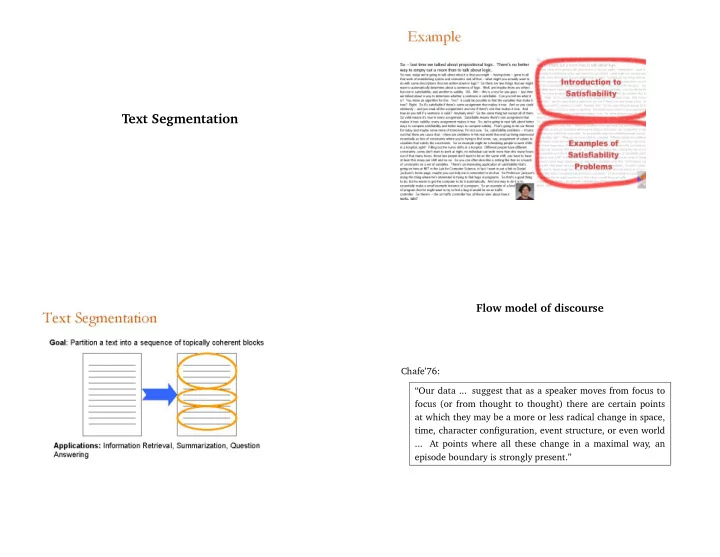
Text Segmentation Flow model of discourse Chafe76: Our data ... - PowerPoint PPT Presentation

Text Segmentation Flow model of discourse Chafe’76: “Our data ... suggest that as a speaker moves from focus to focus (or from thought to thought) there are certain points at which they may be a more or less radical change in space, time, character configuration, event structure, or even world ... At points where all these change in a maximal way, an episode boundary is strongly present.”

Discourse Exhibits Structure! Segmentation: Agreement Percent agreement — ratio between observed agreements and possible agreements • Discourse can be partitioned into segments, which can be A B C connected in a limited number of ways − − − − − − • Speakers use linguistic devices to make this structure explicit + − − − + + cue phrases, intonation, gesture − − − + + + − − − • Listeners comprehend discourse by recognizing this structure − − − – Kintsch, 1974: experiments with recall – Haviland&Clark, 1974: reading time for given/new information 22 8 ∗ 3 = 91% Types of Structure Results on Agreement • Linear vs. hierarchical – Linear: paragraphs in a text – Hierarchical: chapters, sections, subsetions People can reliably predict segment boundaries! Grosz&Hirschbergberg’92 newspaper text 74-95% Hearst’93 expository text 80% • Typed vs. untyped Passanneau&Litman’93 monologues 82-92% – Typed: introduction, related work, experiments, conclusions Our focus: Linear segmentation

Example Stargazers Text(from Hearst, 1994) • Intro - the search for life in space • The moon’s chemical composition • How early proximity of the moon shaped it • How the moon helped life evolve on earth • Improbability of the earth-moon system DotPlot Representation Example Key assumption: change in lexical distribution signals topic change (Hearst ’94) -------------------------------------------------------------------------------------------------------------+ Sentence: 05 10 15 20 25 30 35 40 45 50 55 60 65 70 75 80 85 90 95| -------------------------------------------------------------------------------------------------------------+ • Dotplot Representation: ( i, j ) – similarity between sentence i 14 form 1 111 1 1 1 1 1 1 1 1 1 1 | 8 scientist 11 1 1 1 1 1 1 | 5 space 11 1 1 1 | and sentence j 25 star 1 1 11 22 111112 1 1 1 11 1111 1 | 5 binary 11 1 1 1| 4 trinary 1 1 1 1| 8 astronomer 1 1 1 1 1 1 1 1 | 7 orbit 1 1 12 1 1 | 6 pull 2 1 1 1 1 | 0 16 planet 1 1 11 1 1 21 11111 1 1| 7 galaxy 1 1 1 11 1 1| 4 lunar 1 1 1 1 | 100 19 life 1 1 1 1 11 1 11 1 1 1 1 1 111 1 1 | 27 moon 13 1111 1 1 22 21 21 21 11 1 | 3 move 1 1 1 | 200 7 continent 2 1 1 2 1 | 3 shoreline 12 | Sentence Index 6 time 1 1 1 1 1 1 | 300 3 water 11 1 | 6 say 1 1 1 11 1 | 3 species 1 1 1 | -------------------------------------------------------------------------------------------------------------+ 400 Sentence: 05 10 15 20 25 30 35 40 45 50 55 60 65 70 75 80 85 90 95| -------------------------------------------------------------------------------------------------------------+ 500 0 100 200 300 400 500 Sentence Index

Outline Similarity Computation: Representation Vector-Space Representation SENTENCE 1 : I like apples • Local similarity-based algorithm SENTENCE 2 : Apples are good for you • Global similarity-based algorithm Vocabulary Apples Are For Good I Like you • HMM-based segmentor Sentence 1 1 0 0 0 1 1 0 Sentence 2 1 1 1 1 0 0 1 Segmentation Algorithm of Hearst Similarity Computation: Cosine Measure Cosine of angle between two vectors in n-dimensional space • Initial segmentation � t w y,b 1 w t,b 2 sim ( b 1 , b 2 ) = – Divide a text into equal blocks of k words �� � n t w 2 t =1 w 2 t,b 1 t,b 2 • Similarity Computation SENTENCE 1 : 1 0 0 0 1 1 0 – compute similarity between m blocks on the right and the left of SENTENCE 2 : 1 1 1 1 0 0 1 the candidate boundary √ 1 ∗ 0+0 ∗ 1+0 ∗ 1+0 ∗ 1+1 ∗ 0+1 ∗ 0+0 ∗ 1 sim(S 1 ,S 2 ) = (1 2 +0 2 +0 2 +0 2 +1 2 +1 2 +0 2 ) ∗ (1 2 +1 2 +1 2 +1 2 +0 2 +0 2 +1 2 ) = 0 . 26 Output of Similarity computation: 0.22 • Boundary Detection – place a boundary where similarity score reaches local minimum 0.33

Boundary Detection Evaluation Results • Boundaries correspond to local minima in the gap plot 1 0.9 Methods Precision Recall 0.8 0.7 Random Baseline 33% 0.44 0.37 0.6 Random Baseline 41% 0.43 0.42 0.5 0.4 Original method+thesaurus-based similarity 0.64 0.58 0.3 Original method 0.66 0.61 0.2 20 40 60 80 100 120 140 160 180 200 220 240 260 Judges 0.81 0.71 • Number of segments is based on the minima threshold ( s − σ/ 2 , where s and σ correspond to average and standard deviation of local minima) Segmentation Evaluation More Results Comparison with human-annotated segments(Hearst’94): • 13 articles (1800 and 2500 words) • 7 judges • High sensitivity to changes in parameter values • boundary if three judges agree on the same segmentation point – Parameters: Block size, window size and boundary threshold • Thesaural information does not help – Thesaurus is used to compute similarity between sentences — synonyms are considered to be identical • Most of the mistakes are “close misses”

Outline • Local similarity-based algorithm • Global similarity-based algorithm • HMM-based segmentor

Evaluation Metric: P k Measure Hypothesized segmentation Reference segmentation okay miss false okay alarm P k : Probability that a randomly chosen pair of words k words apart is inconsistently classified (Beeferman ’99) • Set k to half of average segment length • At each location, determine whether the two ends of the probe are in the same or different location. Increase a counter if the algorithm’s segmentation disagree • Normalize the count between 0 and 1 based on the number of measurements taken Notes on P k measure • P k ∈ [0 , 1] , the lower the better • Random segmentation: P k ≈ 0 . 5 • On synthetic corpus: P k ∈ [0 . 05 , 0 . 2] • On real segmentation tasks: P k ∈ [0 . 2 , 0 . 4]

Typed Segmentation • Task: determining the positions at which topics change in a stream of text or speech and identify the type of each segment. • Example: divide newsstream into stories about sports, politics, entertainment, etc. Story boundaries are not provided. List of possible topics is provided. • Straightforward solution: use a segmentor to find story boundaries and then assign to each story a topic label. – Segmentation mistakes may interfere with the classification step. – Combining the two steps can increase the accuracy Outline Types of Constraints • “Local”: negotiations is more likely to predict the topic politics rather than entertaiment • Local similarity-based algorithm • “Contextual”: politics is more likely to start the broadcast than • Global similarity-based algorithm to follow sports • HMM-based segmentor