Temporal-Di ff erence Learning What is MC estimation doing? - - PDF document

Coming Up With Better Policies

We can interleave policy evaluation with policy improvement as before. ⇡0

E

• ! Q⇡0 I
• ! ⇡1

E

• ! · · · I
• ! ⇡⇤ E
• ! Q⇤

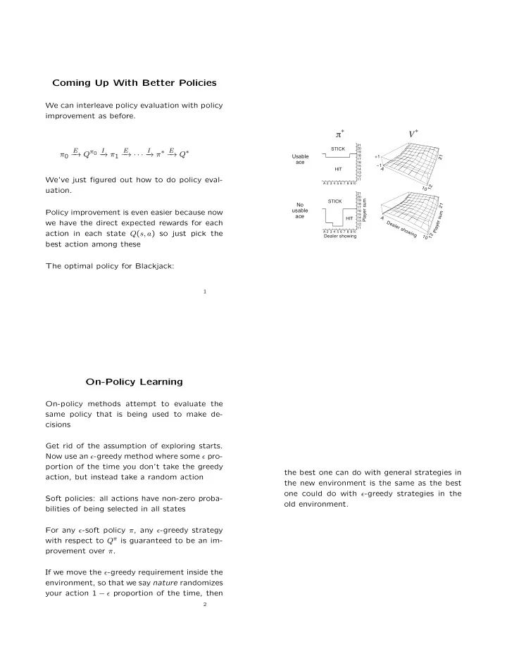
We’ve just figured out how to do policy eval- uation. Policy improvement is even easier because now we have the direct expected rewards for each action in each state Q(s, a) so just pick the best action among these The optimal policy for Blackjack:

1 Usable ace No usable ace

20 10 A 2 3 4 5 6 7 8 9

Dealer showing Player sum HIT STICK

19 21 11 12 13 14 15 16 17 18

π*

10 A 2 3 4 5 6 7 8 9

HIT STICK

20 19 21 11 12 13 14 15 16 17 18

V*

21 1 12 A Dealer showing P l a y e r s u m 1 A 12 21 +1 −1

On-Policy Learning

On-policy methods attempt to evaluate the same policy that is being used to make de- cisions Get rid of the assumption of exploring starts. Now use an ✏-greedy method where some ✏ pro- portion of the time you don’t take the greedy action, but instead take a random action Soft policies: all actions have non-zero proba- bilities of being selected in all states For any ✏-soft policy ⇡, any ✏-greedy strategy with respect to Q⇡ is guaranteed to be an im- provement over ⇡. If we move the ✏-greedy requirement inside the environment, so that we say nature randomizes your action 1 ✏ proportion of the time, then

2

the best one can do with general strategies in the new environment is the same as the best

• ne could do with ✏-greedy strategies in the
• ld environment.

Adaptive Dynamic Programming

Simple idea – take actions in the environment (follow some strategy like ✏-greedy with re- spect to your current belief about what the value function is) and update your transition and reward models according to observations. Then update your value function by doing full dynamic programming on your current believed model. In some sense this does as well as possible, subject to the agent’s ability to learn the tran- sition model. But it is highly impractical for anything with a big state space (Backgammon has 1050 states)

3

Temporal-Difference Learning

What is MC estimation doing? V (st) (1 ↵t)V (st) + ↵tRt where Rt is the return received following being in state st. Suppose we switch to a constant step-size ↵ (this is a trick often used in nonstationary en- vironments) TD methods basically bootstrap off of exist- ing estimates instead of waiting for the whole reward sequence R to materialize V (st) (1 ↵)V (st) + ↵[rt+1 + V (st+1)] (based on actual observed reward and new state) This target uses the current value as an es- timate of V whereas the Monte Carlo target

4

uses the sample reward as an estimate of the expected reward If we actually want to converge to the opti- mal policy, the decision-making policy must be GLIE (greedy in the limit of infinite explo- ration) – that is, it must become more and more likely to take the greedy action, so that we don’t end up with faulty estimates (this problem can be exacerbated by the fact that we’re bootstrapping)

Q-Learning: A Model-Free Approach

Even without a model of the environment, you can learn effectively. Q-learning is conceptually similar to TD-learning, but uses the Q function instead of the value function

• 1. In state s, choose some action a using pol-

icy derived from current Q (for example, ✏-greedy), resulting in state s0 with reward r.

• 2. Update:

Q(s, a) (1↵)Q(s, a)+↵(r+ max

a0

Q(s0, a0)) You don’t need a model for either learning or action selection! As environments become more complex, using a model can help more (anecdotally)

5

Generalization in Reinforcement Learning

So far, we’ve thought of Q functions and utility functions as being represented by tables Question: can we parameterize the state space so that we can learn (for example) a linear function of the parameterization? V✓(s) = ✓1f1(s) + ✓2f2(s) + · · · + ✓nfn(s) Monte Carlo methods: We obtain sample of V (s) and then learn the ✓’s to minimize squared error. In general, often makes more sense to use an

• nline procedure, like the Widrow-Hoff rule:

6

Suppose our linear function predicts V✓(s) and we actually would “like” it to have predicted something else, say v. Define the error as E(s) = (V✓(s) v)2/2. Then the update rule is: ✓i ✓i ↵@E(s) @✓i = ✓i + ↵(v V✓(s))@V✓(s) @✓i If we look at the TD-learning updates in this framework, we see that we essentially replace what we’d “like” it to be with the learned backup (sum of the reward and the value func- tion of the next state: ✓i ✓i + ↵[R(s) + V✓(s0) V✓(s)]@V✓(s) @✓i This can be shown to converge to the closest function to the true function when linear func- tion approximators are used, but it’s not clear how good a linear function will be at approxi- mating non-linear functions in general, and all bets on convergence are off when we move to non-linear spaces. The power of function approximation: allows you to generalize to values of states you haven’t yet seen! In backgammon, Tesauro constructed a player as good as the best humans although it only examined one out of every 1044 possible states. Caveat: this is one of the few successes that has been achieved with function approximation and RL. Most of the time it’s hard to get a good parameterization and get it to work.