[PPT] - TDDC17 Computer systems Robotic architectures Robotics/Perception PowerPoint Presentation

SLIDE 1

Mariusz Wzorek IDA/AIICS

TDDC17 Robotics/Perception II

1 Outline

Sensors - summary
Computer systems
Robotic architectures
Navigation:
Mapping and Localization
Motion planning
Motion control

2 Robotics – application perspective

3 TDDC17 Robotics/Perception II

Application Base Platform Sensors Autonomy, modes of

peration

Computer systems Software architecture Communication:

WiFi, 4G/5G,

dedicated comm links Purpose/Task Environment Budget Mobility:

Wheels, belts,

legs, propellers, rotors? Manipulators:

arms, grippers?

Accuracy Range Reliability Redundancy …

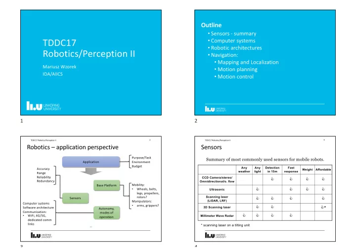
3 Sensors

Summary of most commonly used sensors for mobile robots.

4 TDDC17 Robotics/Perception II

Any weather Any light Detection in 15m Fast response Weight Affordable CCD Camera/stereo/ Omnidirectional/o. flow

C C C C

Ultrasonic

C C C C

Scanning laser (LiDAR, LRF)

C C C C

3D Scanning laser

C C C*

Millimeter Wave Radar

C C C C

* scanning laser on a tilting unit

4

SLIDE 2

Sensors cont’d

5 TDDC17 Robotics/Perception II

waymo.com

5 Sensors cont’d

6 TDDC17 Robotics/Perception II

tesla.com

6 Sensors - common interfaces

analog - voltage level
digital:
serial connections e.g.:
RS232
I2C
SPI
USB
Ethernet
pulse width modulation - PWM
…

7 TDDC17 Robotics/Perception II

7 Outline

Sensors - summary
Computer systems
Robotic architectures
Navigation:
Mapping and Localization
Motion planning
Motion control

8

SLIDE 3

Computer systems

Many challenges and trade-offs!

power consumption
size & weight
computational power
robustness
different operational conditions moisture, temperature, dirt,

vibrations, etc.

cloud computing?

9 TDDC17 Robotics/Perception II

9 Computer systems cont’d

PC104 - standardised form factor

industrial grade
relatively small size
highly configurable
>200 vendors world-wide
variety of components
variety of processors

10 TDDC17 Robotics/Perception II ~10x10cm

10 Computer systems cont’d

Custom made embedded systems

with integrated sensor suite
micro scale, light weight
fitted for platform design

11 TDDC17 Robotics/Perception II

fitted for platform design

11 Computer systems cont’d

Example system design:

12 TDDC17 Robotics/Perception II

!"#$

!"#$!%&'!()*+,-./!
!"!%0!12/!
!"!%0!3456!789:)!

%&#$

!;<<!/&'!()*+,-!===!
!>?@!/0!12/!
!?">!/0!3456!789:)!

'%#$

!;<<!/&'!()*+,-!===!
!>?@!/0!12/!
!?">!/0!3456!789:)!

AB6)8*)B! CD9BE6! FFG!FHIH8! F4-)84! J6)8-4I! F4-)84! (4*! J9IB! K*9B! L4-464!1/2M!NL2CO!L2FCP! 048H-)B89E!(8)55,8)!2I+-)B)8! %(C!1)E)9:)8! Q45)8!14*R)!S9*7)8! /H7,I)! AB6)8*)B!T97)H!C)8:)8! U<>#""V!W98)I)55!0897R)! %C/!/H7)-5!

()8E)X+H*!C)*5H8!C,9B)! FH--,*9E4+H*!/H7,I)! (SF!C)*5H8!C,9B)!

CB)8)H.T959H*! /H7,I)! (HD)8!/4*4R)-)*B!K*9B! AB6)8*)B! 1C>Y>! 2*4IHR! S98)D98)! /9*9GT! 1)EH87)85!

12

SLIDE 4

Ground Robot at AIICS LiU

13 TDDC17 Robotics/Perception II

13

14 TDDC17 Robotics/Perception II

Base platform

Husky unmanned ground

vehicle by Clearpath

run time: up to 3h
Max speed: 1 m/s
Weight: 50 kg
Max payload: 75 kg

14

15 TDDC17 Robotics/Perception II

Robot Arm UR5 – Universal Robotics

Weight: 20.6 kg
Max payload: 5 kg
Working radius: 850 mm
6 DOF

LiDAR (Light Detection and Ranging) sensor - Velodyne

Range: 100m
Vertical FOV: 30deg
Horizontal FOV: 360deg

Battery pack for arm Gripper Gripper – Weiss Robotics

Weight: 1.2 kg
Max payload: 8 kg

15

16 TDDC17 Robotics/Perception II

Network switch Stereo camera Inertial Measurement Unit GPS antenna WiFi router Robot arm power and control system Intel NUC i7 computer GPU – Jetson TK1

16

SLIDE 5

Outline

Sensors - summary
Computer systems
Robotic architectures
Navigation:
Mapping and Localization
Motion planning
Motion control

17 Telesystems/Telemanipulators

18 TDDC17 Robotics/Perception II

Delay

18 Telepresence

Experience of being fully present at live event without actually being there

see the environment through robot’s cameras
feel the surrounding through robot sensors
Realised by for example:
stereo vision
sound feedback
cameras that follow the operator’s head movements
force feedback and tactile sensing
VR system

19 TDDC17 Robotics/Perception II

19 Reactive systems

Robot responses directly to sensor stimuli. Intelligence emerges from combination of simple behaviours. For example - subsumption architecture (Rodney Brooks, MIT):

concurrent behaviours
higher levels subsume behaviours of lower layers
no internal representation
finite state machines

20 TDDC17 Robotics/Perception II

Sense Act

https://www.youtube.com/watch?v=9u0CIQ8P_qk

20

SLIDE 6

Limitations of Reactive Systems

Agents without environment models must have sufficient

information available from local environment

If decisions are based on local environment, how does it take

into account non-local information (i.e., it has a “short-term” view)

Difficult to make reactive agents that learn
Since behaviour emerges from component interactions plus

environment, it is hard to see how to engineer specific agents (no principled methodology exists)

It is hard to engineer agents with large numbers of behaviours

(dynamics of interactions become too complex to understand)

21 TDDC17 Robotics/Perception II

21 Hierarchical Systems

Sensors

22 TDDC17 Robotics/Perception II

Sense

Act Plan

Actuators Extract features combine features into model Plan task Execute task Control motors

22 Hierarchical Systems (Shakey Example)

Shakey (1966 - 1972)

Developed at the Stanford Research Institute
Used STRIPS planner (operators, pre and post conditions)
Navigated in an office environment, trying to satisfy a goal

given to it on a teletype. It would, depending on the goal and circumstances, navigate around obstacles consisting of large painted blocks and wedges, push them out of the way, or push them to some desired location.

Primary sensor: black-and-white television camera
Sting symbolic logic model of the world in the form of first
rder predicate calculus
Very careful engineering of the environment

23 TDDC17 Robotics/Perception II

https://www.youtube.com/watch?v=GmU7SimFkpU

23 Hybrid systems (three-layer architecture)

24 TDDC17 Robotics/Perception II

Sense

Act Plan

24

SLIDE 7

Hybrid systems (Minerva Example)

Tour guide at the Smithsonian's National Museum of American History (1998)

25 TDDC17 Robotics/Perception II

http://www.cs.cmu.edu/~thrun/movies/minerva.mpg

25 Hybrid systems (HDR3 – AIICS/IDA @ LiU Example)

26 TDDC17 Robotics/Perception II

26 Outline

Sensors - summary
Computer systems
Robotic architectures
Navigation:
Mapping and Localization
Motion planning
Motion control

27 Navigation

Mapping – Localization – SLAM – State Estimation – Control

28 TDDC17 Robotics/Perception II

Navigation Mapping

Create a model of the environment. Assumes that we know where the robot and its sensors are.

Localization SLAM Motion Planning Control State Estimation

How do I safely get from point A to B? Estimate position (pose) of a robot in the environment,

r poses of landmarks in the

environment – sensor data can be noisy Where am I? Application of state estimation to calculate robot location (e.g. x, y, orientation - pose). One of the basic functionalities required for any real world deployment:

need to know where

we are

what the

environment looks like Simultaneous Localization and Mapping How do I execute planned motion? E.g. generate control signals to follow planned trajectory (velocity, position commands, etc.)

28

SLIDE 8

0o View from top

LiDAR – recap

Active sensor based on time of flight principle

emits light waves from a laser
measures the time it took for the signal to return to calculate the

distance

29 TDDC17 Robotics/Perception II

29

View from top

LiDAR – recap cont’d

SICK LMS (single line sensor):

Range (d): 80m
Field of View - horizontal (a):

0o-180o

Angular resolution - horizontal (b):

0.25o-1o

30 TDDC17 Robotics/Perception II

a b d View from side

Velodyne Puck (multi-line sensor):

Range (d): 100m
Field of View - horizontal (a):

360o

Angular resolution - horizontal (b):

0.1o-0.4o

Field of View - vertical (g): ±15o
Angular resolution - vertical (f): 2o

g f

30 LiDAR – recap cont’d

31 TDDC17 Robotics/Perception II

Velodyne: https://www.youtube.com/watch?v=WPtHRVdWXSI https://www.youtube.com/watch?v=KxWrWPpSE8I SICK LMS stationary

range data at certain height

SICK LMS with tilt mechanism Velodyne stationary

31 Mapping

Assume we use a mobile robot platform equipped with a LiDAR sensor Simple idea: combine measurement of robot motion with LiDAR sensor readings Measurement of robot motion - state estimation, e.g. odometry, dead reckoning

Simple odometry - wheel encoders that calculate how many times wheels turned
Visual odometry etc. – e.g. optical flow sensor, or use sensor fusion to produce more

accurate estimation of motion There will always be a measurement error when calculating the state - depending on the technique/sensor used it can be smaller or larger

32 TDDC17 Robotics/Perception II

Scan at x0,y0 Scan at x1,y1 Scans added y x

32

SLIDE 9

Mapping cont’d

33 TDDC17 Robotics/Perception II

Based only on odometry + LiDAR range data

33 Scan matching

Calculate rotation and translation between two consecutive LiDAR scans, which will correct for

dometry error.

Iterative Closest Point (ICP) – iteratively minimize the sum of square differences between two pairs of points which are selected from reference and a source scan. Input: reference scan (blue), source scan (red). Output: rotation and translation between reference and source scans.

34 TDDC17 Robotics/Perception II

https://en.wikipedia.org/wiki/Iterative_closest_point

?

34 Mapping cont’d

35 TDDC17 Robotics/Perception II

Based only on odometry + LiDAR range data + scan matching (ICP)

35 Mapping cont’d

36 TDDC17 Robotics/Perception II

Based only on odometry + LiDAR range data + scan matching (ICP)

36

SLIDE 10

Outline

Sensors - summary
Computer systems
Robotic architectures
Navigation:
Mapping and Localization
Motion planning
Motion control

37 Robotic perception

Robot perception viewed as temporal inference from sequences of actions and measurements → dynamic Bayes network of first order Markov process Example: localization - holonomic robot with range sensor, estimate pose while moving next belief state? → Bayesian inference problem

38 TDDC17 Robotics/Perception II

Xt = (xt, yt, q) – state of the robot at time t -> not observable Zt = (range1, range2, range3, …) – sensor reading at time t -> observable At = (vt, wt) – known action executed at time t P(Xt) = P(Xt|z1:t , a1:t-1) – current believe state (captures past) P(Xt+1 |z1:t+1 , a1:t) = ? given P(Xt) and new observation zt+1

38 Graphical Model

39 TDDC17 Robotics/Perception II

known actions unknown sensor readings M known map

39 Recursive filtering equation

using Bayes’ rule, Markov assumption, theorem of total probability Motion model: deterministic state prediction + noise Sensor model: likelihood of making observation zt+1 when robot is in state Xt+1

40 TDDC17 Robotics/Perception II

P(Xt+1 |z1:t+1 , a1:t) = ! P(zt+1 |Xt+1) ∫ P(Xt+1 | xt, at) P(Xt | z1:t, a1:t-1) dxt sensor model motion model previous believe state

40

SLIDE 11

Motion and sensor model

Assume Gaussian noise in motion prediction, sensor range measurements

41 TDDC17 Robotics/Perception II

41 Graphical Model

42 TDDC17 Robotics/Perception II

known actions unknown sensor readings sensor model motion model M known map

42 Localization algorithms

Particle filter (Monte Carlo localization):

belief state - a collection of particles that correspond to states
belief state sampled, each sample weighted by likelihood it assigns to

new evidence, population resampled using weights Kalman filter:

belief state - a single multivariate Gaussian
each step maps a Gaussian into a new Gaussian, i.e. it computes a new

mean and covariance matrix from the previous mean and covariance matrix

assumes linear motion and measurement models (linearisation

→extended KF)

43 TDDC17 Robotics/Perception II

43 Global Localization (Particle Filter Examples)

44 TDDC17 Robotics/Perception II

P(Xt+1 |z1:t+1 , a1:t) = ! P(zt+1 |Xt+1)

∫ P(Xt+1 | xt, at) P(Xt | z1:t, a1:t-1) dxt

sensor model motion model previous believe state

44

SLIDE 12

Global Localization (Particle Filter Examples)

45 TDDC17 Robotics/Perception II

Intuitive explanation:

initialize particles
execute known action
apply motion model
update particle

weights based on sensor model

resample based on

weights

repeat

45 Global Localization (Particle Filter Examples)

46 TDDC17 Robotics/Perception II

After several iterations – two likely robot position estimates: After more iterations – converged to a single robot position estimation:

46 Global Localization (Particle Filter Examples; sonar vs laser)

47 TDDC17 Robotics/Perception II

47 Extended Kalman Filter (EKF) - example

48 TDDC17 Robotics/Perception II

48

SLIDE 13

EKF example

49 TDDC17 Robotics/Perception II

49 SLAM

Localization: given map and observed landmarks, update pose distribution Mapping: given pose and observed landmarks, update map distribution SLAM: given observed landmarks, update pose and map distribution Probabilistic formulation of SLAM: add landmark locations L1, . . . , Lk to the state vector, proceed as for localization Problems:

dimensionality of map features has to be adjusted dynamically
identification of already mapped features

50 TDDC17 Robotics/Perception II

50 SLAM Example

51 TDDC17 Robotics/Perception II

https://youtu.be/F8pdObV_df4 http://wiki.ros.org/hector_slam

51 Outline

Sensors - summary
Computer systems
Robotic architectures
Navigation:
Mapping and Localization
Motion planning
Motion control

52

SLIDE 14

Motion Planning

Motion types:

point-to-point
compliant motion (screwing, pushing boxes)

Representations: configuration space vs workspace Kinematic state: robot’s configuration (location, orientation, joint angles), no velocities, no forces Path planning: find path from one configuration to another Problem: continuous state space, can be high-dimensional

53 TDDC17 Robotics/Perception II

53 Motion Planning - representations

Workspace - physical 3D space (e.g. joint positions) Robot has rigid body of finite size Well-suited for collision checking Problem: linkage constraints (not all workspace coordinates attainable) makes path planning difficult in workspace Configuration Space (C-space) - space of robot states (e.g. joint angles) Robot is a point, obstacles have complex shapes Problem: tasks are expressed in workspace coordinates, obstacle representation problematic

54 TDDC17 Robotics/Perception II

54 Workspace vs. Configuration Space

55 TDDC17 Robotics/Perception II

55 Workspace vs. Configuration Space

56 TDDC17 Robotics/Perception II

56

SLIDE 15

Cfree

Workspace vs. Configuration Space

57 TDDC17 Robotics/Perception II

O Cobs O

x x y y

q – a robot configuration e.g. (x1,y1,q1) A(q) – set of points on the robot in configuration q .

x1 y1 q1 x1 y1 A(q)

W – workspace world either ℝ2 or ℝ3 O – obstacle region, O⊂W C – all possible robot configurations Cobs = {q : q ∈ C and A(q) ∩ O ≠ {} } Cfree=C – Cobs

57 Motion Planning - representations

Free space (attainable configurations) ->occupied space (not attainable configurations, obstacles) Planner may generate configuration in configuration space, apply kinematics and check in workspace for obstacles

58 TDDC17 Robotics/Perception II

Workspace Configuration Space

Inverse kinematics (often hard and ill-posed problem) Forward Kinematics (simple, well-posed problem)

58 Path Planning

Basic problem: convert infinite number of states into finite state space Cell decomposition:

divide up space into simple cells,
each of which can be traversed “easily”

Skeletonization:

identify a finite number of easily connected points/lines
form a graph such that any two points are connected by a path

Graph search and colouring algorithms Assumptions: motion deterministic, localization exact, static scenes Not robust with respect to small motion errors, does not consider limits due to robot dynamics

59 TDDC17 Robotics/Perception II

59 Cell Decomposition

60 TDDC17 Robotics/Perception II

Grayscale shading - cost from the grid cell do the goal

60

SLIDE 16

Cell Decomposition

Problem: may be no path in pure free space cells Soundness (wrong solution if cells are mixed) vs. Completeness (no solution if only pure free cells considered) Solution: recursive decomposition of mixed (free+obstacle) cells or exact

decomposition. Doesn’t scale well for higher dimensions.

61 TDDC17 Robotics/Perception II

61 Skeletonization

Visibility graphs: find lines connecting obstacle vertices through free space, build and search graph; not for higher dimensions Voronoi graphs: find all points in free space equidistant to two or more

bstacles, build and search graph; maximizes clearance, creates unnecessarily

large detours, does not scale well for higher dimensions Sample-based path planners. Probabilistic roadmaps (PRM):

generate randomly large number of configurations in free space, build

graph (construction phase)

search graph (query phase)

Rapidly exploring Random Trees (RRT):

generate a tree rooted in start configuration by random sampling of free

space until goal configuration is reached (query phase) Scales better to higher dimensions but incomplete

62 TDDC17 Robotics/Perception II

62 Visibility and Voronoi Graph

63 TDDC17 Robotics/Perception II

63 PRM and RRT planning procedure example

64 TDDC17 Robotics/Perception II

64

SLIDE 17

PRM Example (construction phase)

65 TDDC17 Robotics/Perception II

Generate random configurations Make connections Generate random configurations Resulting free space graph representation

65 PRM Example (query phase)

66 TDDC17 Robotics/Perception II

Add start and goal configurations to the roadmap A* search (+optional postprocessing)

start goal start goal start goal

66 PRM Example

67 TDDC17 Robotics/Perception II

67 RRT

68 TDDC17 Robotics/Perception II

https://en.wikipedia.org/wiki/Rapidly-exploring_random_tree RAND_CONF – samples random configuration from free space qrand. NEAREST_VERTEX – find qnear i.e. the closest vertex in existing graph G from qrand. NEW_CONF – select new configuration qnew by moving at incremental distance Dq from qnear in the direction of qrand.

qrand1 qnear qrand2 qnew1 qnew2 Dq Dq

Demo: https://demonstrations.wolfram.com/RapidlyExploringRandomTreeRRTAndRRT/

68

SLIDE 18

RRT*

Asymptotically optimal: Converges to the optimal solution as more and more milestones are sampled.

69 TDDC17 Robotics/Perception II

https://www.youtube.com/watch?v=YKiQTJpPFkA

69 PRM/RRT - Post Processing Example

Example curve replacement and path optimization:

70 TDDC17 Robotics/Perception II

Transformation from linear to cubic (smooth) path segments: Alignment of nodes for improved path quality:

70 Outline

Sensors - summary
Computer systems
Robotic architectures
Navigation:
Mapping and Localization
Motion planning
Motion control

71 Motion Control

Path following involves forces: friction, gravity, inertia,
Dynamic state: kinematic state + robot’s velocities
Transition models expressed as differential equations
Path planner assumes robot can follow any path
Robot’s inertia limits manoeuvrability
Problem: including dynamic state in planners makes motion planning

intractable

Solution: simple kinematic planners + low-level controller for force

calculation

Other solution: motion control without planning: potential field and reactive

control

72 TDDC17 Robotics/Perception II

72

SLIDE 19

Controllers

Techniques for generating robot controls in real time

using feedback from the environment to achieve a control

bjective
Reference controller: keep robot on pre-planned path

(reference path)

Optimal controller: controller that optimises a global cost

function, e.g. optimal policies for MDPs

Stable: small perturbations lead to bounded error between

robot and reference signal

Strictly stable: able to return to reference signal

73 TDDC17 Robotics/Perception II

73 Closed-loop control

Performance of controller:

stability
overshoot ← inertia
steady-state error ← friction
rise time
settling time

P controller:

74 TDDC17 Robotics/Perception II

74 PID Example

75 TDDC17 Robotics/Perception II

x0=0; v0=0 xgoal=15 e(t0)=xgoal-x0=15 present past future

75 Closed-loop control

PD controller:

decreases overshoot
decreases settling time

PID controller:

eliminates steady-state error

76 TDDC17 Robotics/Perception II

76

SLIDE 20

Closed-loop control

77 TDDC17 Robotics/Perception II

P control: KP= 1.0 P control: KP= 0.1 PD control: KP= 0.3 KD=0.3

77 Model Predictive Control

1. At time k, solve open loop optimal control problem over a specified finite time horizon 2. Apply first input 3. At time k+1, repeat from step 1.

78 TDDC17 Robotics/Perception II

https://en.wikipedia.org/wiki/Model_predictive_control

78 Model Predictive Control

79 TDDC17 Robotics/Perception II

https://www.youtube.com/watch?v=dL_ZFSvLXlU Optimizer Predictor (Model)

Reference trajectory Predicted outputs +

Future errors

Process

Cost function Constraints Output Future inputs MPC Predictor/Model: fundamental or empirical Constraints e.g. on inputs, outputs, state are respected

79 MPC – simple example

80 TDDC17 Robotics/Perception II

https://medium.com/@david010/vehicle-mpc-controller-33ae813cf3be https://github.com/cipher982/MPC-vehicle-controller

80

SLIDE 21

MPC and Learning

81 TDDC17 Robotics/Perception II

https://www.youtube.com/watch?v=QYYknZ20Zcw https://www.youtube.com/watch?v=xa53w1tyZl0 https://doi.org/10.3384/diss.diva-163419

81 MPC and Learning

82 TDDC17 Robotics/Perception II

https://www.youtube.com/watch?v=QYYknZ20Zcw https://www.youtube.com/watch?v=xa53w1tyZl0 https://doi.org/10.3384/diss.diva-163419