TCP Protocol CS/ECpE 5516 -- Computer Networks Changes from - - PDF document

CS/EE 5516 - Lecture 10

• 1-

Spring 1998 1

TCP Protocol

CS/ECpE 5516 -- Computer Networks

Changes from original version marked by vertical bar in left margin.

References:

• Peterson & Davie, Computer Networks, Ch. 5
• Comer, Internetworking with TCP/IP, 2
• nd. Edition, Vol. I, Ch. 12
• Stevens, UNIX Network Programming

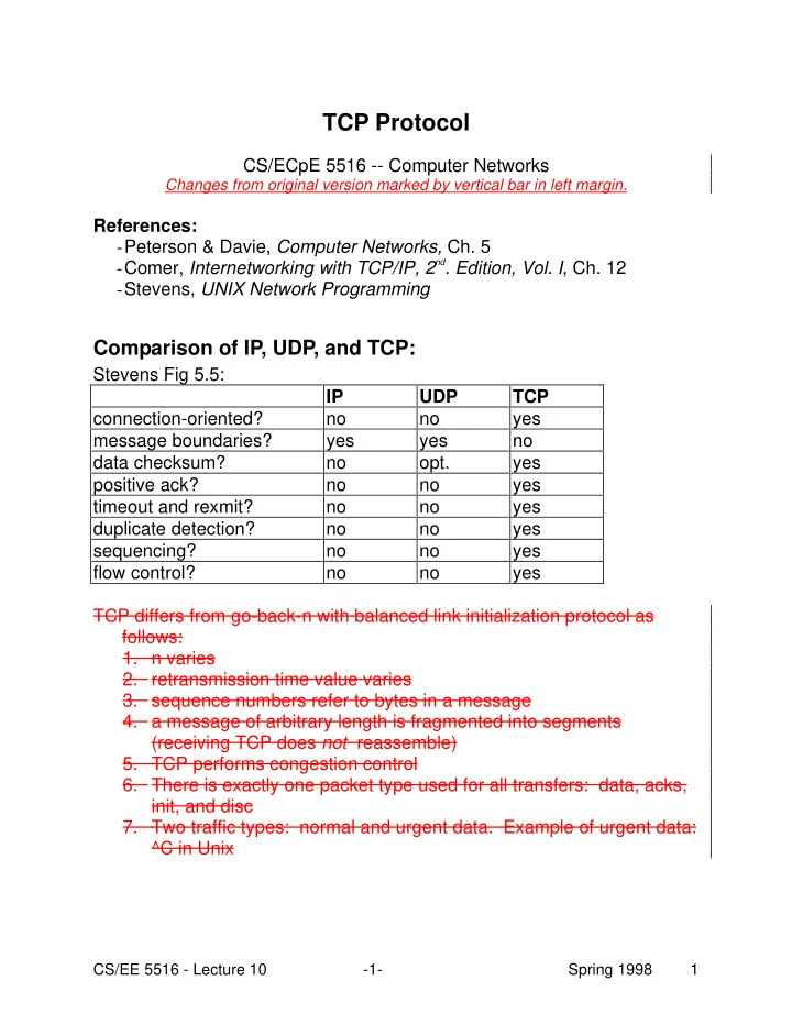
Comparison of IP, UDP, and TCP:

Stevens Fig 5.5: TCP differs from go-back-n with balanced link initialization protocol as follows:

• 1. n varies
• 2. retransmission time value varies
• 3. sequence numbers refer to bytes in a message
• 4. a message of arbitrary length is fragmented into segments

(receiving TCP does not reassemble)

• 5. TCP performs congestion control
• 6. There is exactly one packet type used for all transfers: data, acks,

init, and disc

• 7. Two traffic types: normal and urgent data. Example of urgent data:

^C in Unix IP UDP TCP connection-oriented? no no yes message boundaries? yes yes no data checksum? no

• pt.

yes positive ack? no no yes timeout and rexmit? no no yes duplicate detection? no no yes sequencing? no no yes flow control? no no yes

CS/EE 5516 - Lecture 10

• 2-

Spring 1998 2

Terminology:

How TCP partitions a message into segments: MSS (maximum segment size) is usually no larger than the MTU-2*20. (The term 2*20 is for the TCP and IP headers.) For Ethernet, MSS=1500-2*20 = 1460.

CS/EE 5516 - Lecture 10

• 3-

Spring 1998 3

TCP header format (Comer Fig. 12.7)

• 20 byte header if OPTIONS not used (So 1500-20-20=1460 is MSS

for ethernet)

• There are no separate ACK/DATA segments. TCP normally does

not generate an ACK for received data. Thus ACK is piggybacked

• n DATA.
• Done simply by ACK Number field in every TCP header. This

is the number of the octet that the source expects to receive next (in other words, one more than the largest, contiguous byte number received).

• When TCP receives incoming segment, it waits for outgoing

data, and piggybacks ACK. If no outgoing data for a while, TCP will generate a zero-data length outgoing segment in which to piggyback the ACK.

• HLEN (header length in 32 bit words) is required due to variable

length header

• Code bits (they help distinguish data/ack/init/disc packets):
• URG

urgent pointer field valid

• ACK

ack field is valid

• PSH

this segment requests a push

• RST

reset connection

• SYN

synchronize sequence numbers

• FIN sender has reached end of byte stream
• Note: no special control segments used to establish, release

connection; use ACK, RST, SYN, FIN bits in normal segment

• Finite state machine used for connection establishment/release

(Comer Fig. 12.13)

• CHECKSUM is for header + data
• WINDOW is receiver advertisement
• URGENT POINTER - specifies position in data where urgent data

ENDS, if URG bit is set

CS/EE 5516 - Lecture 10

• 4-

Spring 1998 4

Bit (left to right) Meaning if bit set to 1 URG Urgent pointer field is valid ACK Acknowledgement field is valid PSH This segment requests a push RST Reset the connection SYN Synchronize sequence numbers FIN Sender has reached end of its byte stream (Figure 12.8)

CS/EE 5516 - Lecture 10

• 5-

Spring 1998 5

Variable Window Size (n in Go Back-n) (Comer 12.10)

Overview of TCP Window Two windows:

• Sender window
• Receiver window

Sending window: 11 12 13 14 15 16 17 18 19 Sender maintains three pointers:

• lower edge
• boundary between sent and unsent octets
• upper edge

Behavior:

• Lower and upper edges advance slowly
• Boundary pointer advances rapidly (as fast as sender can transmit)
• Boundary pointer might cycle if retransmission occurs

Goal:

• Lower and upper window edges advance quickly enough so that

boundary never hits upper edge!

• If this happens, the sliding window lets the sender transmit at max

throughput! Receiving Window Receiver has a fixed amount of buffer space. Receiver at any moment has part filled, part unfilled. May have wholes. Receiver periodically releases a contingous prefix to upper layer protocol. 1 2 3 5

CS/EE 5516 - Lecture 10

• 6-

Spring 1998 6

TCP differs from go-back-n with balanced link initialization protocol as follows:

• 1. n varies
• 2. Retransmission time value varies
• 3. Sequence numbers refer to bytes in a message
• 4. A message of arbitrary length is fragmented into segments

(receiving TCP does not reassemble)

• 5. TCP performs congestion control
• 6. Just one packet type used for all transfers: data, acks, initialization,

and disconnect

• 7. Two traffic types: normal and urgent data. Example of urgent data:

^C in Unix

CS/EE 5516 - Lecture 10

• 7-

Spring 1998 7

TCP window solves 3 problems (vs. Comer’s 2 reasons)

• 1. Throttles fast sender
• 2. Provides efficient transmission
• 3. Provides congestion management mechanism

Congestion = intermediate hops are saturated with traffic

• Good TCP implementation help reduce congestion
• Poor TCP implementation can introduce packets to subnet during

congestion period and cause internet breakdown. What does the “window advertisement” in the TCP header mean?

• The i-th ack sent contains:
• RNi = acknowledgement: octet that receiver next expects
• Wi = window advertisement: receiver’s current free buffer size

Initially: W0 = receiver’s buffer size, in bytes

CS/EE 5516 - Lecture 10

• 8-

Spring 1998 8

• Each time an ack (number I) is sent:

Missing formula! Thus the receiver does not contradict previous advertisements (e.g., reduce the sender’s upper window edge)

• Sender sets its upper window edge to a value <= RNi + Wi
• Thus sender sets n in go-back-n to a value <= Wi
• The “<” is due to congestion management, explained later.

Sender only increases its upper window edge if receiver chooses

W W RN RN W RN RN RN RN

i i i i i i i i i

= = − − >   

− − − − − 1 1 1 1 1

if max current free buffer space if ( , ( )

CS/EE 5516 - Lecture 10

• 9-

Spring 1998 9

Example (illustration of receiving TCP)

Suppose that …

• the original window advertisement when connection opened

was 8

• the application on the receiving host does not remove any data

from receiver TCP Step ACK i-1: Receiver is waiting for octets 4, 6, and 7. Thus ACK i-1 contains:

• RNi-1

= 4

• Wi-1

= 4 Step ACK i: Receiver gets receives

• ctet 4.

Thus ACK i contains:

• RNi = 6
• Wi = 2

Alternate for step ACK i: If the receiver’s layer 5 removed bytes 0 and 1, then

• Wi = 4

General Algorithm:

• When ACK i is sent:

Thus the receiver does not contradict previous advertisements (e.g., reduce the sender’s upper window edge)

• Sender sets its upper window edge to a value <= RNi

+ W i

• Thus sender sets n in go-back-n to a value <= Wi

1 2 3 5 1 2 3 4 5

W W RN RN W RN RN RN RN

i i i i i i i i i

= = − − >   

− − − − − 1 1 1 1 1

if max current free buffer space if ( , ( )

CS/EE 5516 - Lecture 10

• 10-

Spring 1998 10

• The “<” is due to congestion management, explained later.
• Sender only increases its upper window edge if receiver chooses

WI

• W

I-1

> RN

I

• RN

I-1

.

CS/EE 5516 - Lecture 10

• 11-

Spring 1998 11

• Q. Receiver can advertise a window size of zero to stop sender.

CCan you think of any exceptions to this rule, where the sender sstill sends segments even though the window size is zero? A.

• Sender can periodically try sending data in case subsequent non-zero

advertisement was lost.

• Sender can send data with urgent flag set to inform receiver that

urgent data is available.

• To avoid deadlock: Sender can periodically try sending data in case

subsequent non-zero advertisement was lost.

• 1. Window size = 0
• 2. Receiver buffer space is freed
• 3. Receiver sends segment with advertisement of non-zero to

sender; segment is lost. Receiver will not try to send more segment if there is no data going in reverse direction (from receiver to sender).

• 4. Sender will wait forever for a non-zero window unless sender is

allowed to send a segment. Q: We claimed earlier that "receiver does not contradict previous advertisements." Thus Why is RNi + Wi must be monotonically increasing. Why?? A:

• RNi obviously is monotonically increasing.
• Wi is not obviously monotonically increasing. However, Wi can

decrease by at most the amount RNi increases (because receiver never reduces total buffer space)

CS/EE 5516 - Lecture 10

• 12-

Spring 1998 12

TCP ACK and Retransmission (Comer [12.15])

Recall:

• RN = next octet expected by receiver
• SN, RN header fields refer to octet # in stream, not a segment number
• Q. Why does TCP use octet number, not segment number, for RN &

SN?

• A. TCP spec allows retrasmitted segment to include more data than
• riginal copy! (Perhaps retransmitted packet did not originally contain

a full frame’s worth of data, and at time of retransmission, sender’s layer 5 passed down more data.) Timeouts and Retransmission (Comer [12.16]) Why can’t the timeout value be fixed in TCP? (Comer [12.16]) 1) Unlike DLC, TCP is used over various delay/BW networks. There’s no a priori knowledge of a "good" timeout value. 2) Unlike DLC, congestion requires dynamic changes to retransmission timeout (TO) value 3) Every connection has its own TO value [Fig 12.10 – graph of round trip time vs. wall clock time].

• Q. Why does every connection have its own TO value?
• A. Two different connections may be between two different hosts in the

Internet, and thus round trip time (RTT) is probably different.

CS/EE 5516 - Lecture 10

• 13-

Spring 1998 13

TCP’s Adaptive Retransmission Algorithm

• TCP monitors each connection, and deduces reasonable TO value
• TO = ß * RTT

(ß = 2 in early TCP spec)

• RTTi is estimated round trip time of a segment, after segment i was

ack’d. Each time ack is received: RTTi = α* RTTi-1 + (1 - α) * RTTlast_segment (1)

• Typical values [Karn & Partridge 1987]:
• α = 0.875
• β = 2

Alternatives to pre-1987 TCP's α, ß values 1) Iif you see a RTTlast_setg ment that’s bigger than your estimated RTTi, switch to a smaller α to adapt more quickly to development of

• congestion. (Idea due to [Mills].)

2) Vary ß based on observed variance in RTTlast_segment. (Due to [Jacobson] - more later.)

α near 1 immune to single segment with long delay near 0 RTTi tracks changes to RTTlast -set rapidly ⇒ ⇒   

CS/EE 5516 - Lecture 10

• 14-

Spring 1998 14

Why choosing ß is hard [Karns and Partridge 87]

• A bad choice of RTT is the median of RTT samples:

Then 1/2 of all packets will be timed out and retransmitted, thereby increasing network load.

• Choice m- Must balance conflict between:
• Individual user throughput
• A sSmall β (β slightly larger than 1) detects packet loss

quickly.

• Overall network efficiency (
• A lLarge β avoids unnecessary retransmissions.
• Ideally,: cC

hoose β so that TO is an upper bound

• n RTTlast_segment
• A bad choice of RTT is the median of RTT samples:

Then 1/2 of all packets will be timed out and retransmitted, thereby increasing network load.

• Mills says RTTlast_segmentg has Poisson distribution, but with brief

periods of high delay.

CS/EE 5516 - Lecture 10

• 15-

Spring 1998 15

Accurate Measurement of RTT samples ([Comer 12.17]) 1) Why can’t you just subtract time segment is sent from time ack is received to compute RTT?

• A. If loss occurs, there is no longer a 1:1 correspondence between sent

segments and acks. This is acknowledgement ambiguity. Example: 1) Sender transmits segment at time t0. 2) Timeout pops. 3) Sender re-transmits segment at t1. 4) Sender receives ack for a segment at t2. Is ack for segment sent at t0 or t1? t0 t1 t2 S R ? ? Should RTT be a) t2 - t0 b) t2 - t1

CS/EE 5516 - Lecture 10

• 16-

Spring 1998 16

Problem with (a) [see picture below]:

• Could cause RTTi to grow w/o bound:
• You send first segment at t0.
• Datagram containing segment is lost.
• You send second segment at t1.
• You get ack for second segment at t2.
• You use t2-t0 as RTT sample. That’s too long.
• Now you send second segment at t3.
• Datagram containing second segment is lost.
• You now wait a long time before retransmitting – namely for t2-t0.
• You get ack at t4. You now use t4-t3 >> t2-t0 as sample.
• Continuing like this, RTT grows without bound!

t0 t1 t2 R X t3 t4 X t2-t0 TO = β(t2-t0) RTT increases!

CS/EE 5516 - Lecture 10

• 17-

Spring 1998 17

Problem with (b):

• RTT estimate is too small if a loss did occur; timer will pop too early in

future

• You send first segment at t0.
• Timer pops and you retransmit at t1.
• Suddenly the ack for datagram sent at t0 arrives at time t2; you use

t2-t1 (which could be nearly 0!) as RTT sample. That’s much too short.

• You now send second datagram at t3.
• Your timer is too small, so you retransmit at t4, very soon after t3 –

the second segment has no hope of being ack’d before your timer pops. t0 t1 t2 R t3 Two unneeded retransmissions RTT sample t2-t1 too small! Original TO -

• Every segment is now transmitted at least twice, even though no loss
• ccurs!
• Steady state that’s been observed for this situation:

RTT = (1/2) RTTactual + ε

CS/EE 5516 - Lecture 10

• 18-

Spring 1998 18

Ambiguity Problem Solution:

• Ignore RTT samples of any packet that was retransmitted.
• Problem:
• Works ok if actual RTT changes slowly.
• But sudden spike in actual RTT will cause retransmission for all

subsequent packets:

• The high RTT of retransmitted packets is ignored.
• Hence sender is stuck with too small a timeout value
• This in turn wastes network capacity when it can least afford it -

during periods of congestion.

• It’s like pouring gas on a fire!

CS/EE 5516 - Lecture 10

• 19-

Spring 1998 19

[C 12.18] Karn’s algorithm and timer backoff (Karn’s, Partridge, 1988)

• Virtually all TCP implementations (old and new) increase timeout upon

retransmission. If 2 timeouts for same packet occur, timeout is increased still further.

• Increasing timeout = backoff
• Example (early TCP)
• BSD 4.3 has table of factors for each successive retransmission
• Simply double timeout
• Alternative to backoff:
• Set timeout excessively high, so that no packet could survive

retransmission.

• This is a bad solution:

It gives poor user throughput over a lossy path. Karn’s Algorithm:

• When an ack arrives for a packet sent >1 time, do not use it to compute
• RTT. Instead, back off timer.
• Retain backed off time for subsequent packets until a packet is sent

and ack’d w/o retransmission.

• At this point, recalculate TO from RTTlast_segment using formula

(1).

• This insures RTTi will gradually converge to new, higher actual

round trip time. Q: How quickly does RTT converge to true value? A: In worst case, need just 6 good samples of RTTlast_segmentg for RTTi

CS/EE 5516 - Lecture 10

• 20-

Spring 1998 20

to converge on actual value, for ß = 2, α = .87. [Karn, Partridge 88]

CS/EE 5516 - Lecture 10

• 21-

Spring 1998 21

TCP Modifications due to [Jacobson, 1987]

• New Post-1987 TCP spec arose from

due to congestion collapse in F(fall 86) in Internet: Throughput of 400 yard, 3-hop path dropped from 32kbps to 40bps.

• New principle: Conservation of packets:
• At equilibrium, "A new packet should not enter until an old one

leaves"

• Equilibrium = "Running stably with a full window of data in transit"
• New packets are "clocked in" by returning acks.
• Self clocking systems automatically adjust to BW & delay variance

and have a wide dynamic range

• (TCP spans 1200bps to 800mbpsGbps)

Observation: Congestion collapse occurs if conservation of packets is violatedfails. This Failure occurs due to one of 3 reasons: Failure 1) Connection doesn’t get to equilibrium Failure 2) Sender injects new packet before old packet exits. Failure 3) Equilibrium can’ t be reached because of resource limits along pathis upset when network congestion develops.

CS/EE 5516 - Lecture 10

• 22-

Spring 1998 22

Solution to Failure 1 - Slow start (Peterson/Davie section 6.3.2) Pre-1987: :

• If you suddenly start a file transfer for a host connected to a 10Mbps

Ethernet and through a 56 Kbps gateway to the destination, you begin flooding Ethernet at 10 Mbps: 200 x (gateway BW).

• This causes continuous retransmissions.

.

• See [Jacobson, Fig. 3] – two Sun’s on Ethernets connected by

230.4Kbps microwave link:

• Dot = 512 byte packet
• Vertical lines of dots = retransmissions
• Receiver buffer space yielded 20KBps max throughput
• Only 35% of available BW was used (distance from dotted line)
• Packets 54 to 58 were sent 5 times each!
• See [Jacobson, Fig. 4] – Fig. 3 after applying slow start algorithm

(described below).

• Achieves 16 Kbps out of possible 20KbBps. (Note

2 second offset in lower left due to slow start; this reduces bandwidth to 20Kbps, still twice Fig. 3.)

• Twice the throughput of Fig. 3, and 75% of max throughput (16 vs.

20KBps)

CS/EE 5516 - Lecture 10

• 23-

Spring 1998 23

So, there needs to be a way to "discover" bottleneck path BW. This is slow start:

• Add a congestion window, CWND, to each connection.
• When starting or restarting after a retransmission, set CWND to
• ne packet.
• On each ack for new data, increase CWND by one packet.
• The value of n (in Go Back n) at sender is

min(CWND, receiver’s advertised window in last header received).

CS/EE 5516 - Lecture 10

• 24-

Spring 1998 24

Example [Jacobson 1988, fig 2] Legend: Ack Data R

• ne round trip time
• ne packet time

1

R

2 3 1

2R

4 5 2 6 7 3

R

8 9 4 10 5 11 12 6 14 7 15 13 Opening a window of size 16: 1 3

• Horizontal direction is time.
• Continuous time line has been chopped into one-round-trip-time pieces stacked

vertically with increasing time going down the page.

• As each ack arrives, two packets are generated:
• 1. one for the ack (the ack says a packet has left the system, so a new packet is

added to take its place)

• 2. one because an ack opens the congestion window by one packet.
• Add-one-packet-to-window policy opens the window exponentially in time (3 round

trips => window=2

3=16).

• If local net is much faster than long haul net, ack’s two packets arrive at bottleneck

at essentially the same time.

• These two packets are shown stacked on top of one another (indicating that
• ne of them would have to occupy space in the gateway’s short term queue).

CS/EE 5516 - Lecture 10

• 25-

Spring 1998 25

• Thus, the short term queue demand on the gateway is increasing exponentially
• Opening a window of size W packets will require W/2 packets of buffer capacity

at the bottleneck.

CS/EE 5516 - Lecture 10

• 26-

Spring 1998 26

Solution to Failure 2 (Peterson/Davie section 6.4.3) (Sender injects new packet before old packet exits):

• (2)Failure 2 only occurs if there’s unnecessary retransmission
• Thus it's critical to accurately estimate RTT algorithm
• New idea: estimate variance of RTT, denoted by σRTT

Let ρ denote utilization (0-100%) of network. By queuing theory, RTT and σRTT both scale proportionally to 1/(1-ρ).

• Thus if ρ= 75%, RTT will vary by a factor of ± 2σRTT, or ± 2

.4, or a range

• f (-8, +8), or 16. Wow!
• Using early TCP standard’s suggestion of ß = 2 means TCP can adapt
• nly to of ρ ≤ 30%. So if load ρ goes above 30%, unnecessary

retransmissions occur. Responding to high variance in delay (Comer [12.19]) 1989 TCP spec requires estimation of mean as well as variance in RTT. Let

• DEV denote standard deviation
• δ denote a weighting factor between 0 and 1 that controls how

quickly the new sample affects the weighted average; typically 1/8 Then RTTi = RTTi-1 + δ (Sample - RTTi-1) [δ=1 means adapt instantly] Note: above is faster to compute than RTTi = α* RTTi-1 + (1 - α) * Sample Use standard deviation in place of ß to estimate Timeout (was ß * RTTi)

CS/EE 5516 - Lecture 10

• 27-

Spring 1998 27

Timeouti = RTTi + 2*DEVi , where DEVi = DEVi-1 + δ (|Sample - RTTi-1| - DEVi-1) Above formula doesn’t use true std. deviation formula to avoid time consuming terms (e.g., squaring an integer) Why timeouti = DEVi * RTTi is better than ß(=2) * RTTi:

RTTi DEV+RTTi 2RTTi pdf of RTTi RTTi DEV+ RTTi 2RTTi pdf of RTTi

• RTT and σRTT both grow with network load, denoted ρ (0 ≤ ρ ≤ 1).

Compare Figs. 5 & 6 in [Jacobson]:

• Fig. 5 is ß(=2) * RTTi
• Fig. 6 is DEVi * + RTTi

Summary:

• RTT is updated only for segments not retransmitted
• Timeout is doubled whenever segment timer pops
• When timeout is updated

CS/EE 5516 - Lecture 10

• 28-

Spring 1998 28

• > higher std. dev leads to large timeout
• > small std. dev. leads to small timeout

CS/EE 5516 - Lecture 10

• 29-

Spring 1998 29

Solution to Failure 3: Congestion Window [Comer 12.20] Dynamic setting of CWND (solution to 2 and 3) 1 Congestion collapse Offered load Must have a way to quench sources when operating in this region. TPut Q: Why does curve decline? A: Transport protocols retransmit when timers pop. Long queue delays -> lots of times pop -> most datagrams are retransmissions. So we use retransmission as a “signal” that network is congested:

• Decrease utilization if signal is received
• Increase utilization otherwise.

Note: retransmission is a good signal because all networks deliver it! No special bits need to be added to protocols or implementations.

CS/EE 5516 - Lecture 10

• 30-

Spring 1998 30

Multiplicative Decrease:

• Add to the state of each TCP connection a new state variable:

CWND (Congestion Window)

• Sender’s window size is min(CWND, Window-Advertisement)
• In steady state, on non-congested connection:

CWND

i = Receiver’s window

• When congestion is present, how does TCP know what value to use for

CWND?

• TCP uses the occurrence of a timeout as a signal for congestion.
• So Oon congestion

(packet retransmission ( congestion), we decrease

• CWND. But by how much?
• During congestion, queue lengths at routers increase exponentially

(recall that RTT scales proportionally to 1/(1-ρ)); thus we must decrease window size exponentially: SSTHRESH = SSTHRESH * D (SSTHRESH is explained later) CWND = CWND/2 1

• This reduction of CWND throttles sender.

where D = 1/2

• Also double timeout value upon each retransmission, by (Karn’s

algorithm)

• This reduction of CWND throttles sender.

Additive Increase

• If you’re sharing network link with one other person, you each will get

i Called CongestionWindow in Peterson and Davie; terminology used here is Van Jacobson’s.

CS/EE 5516 - Lecture 10

• 31-

Spring 1998 31

50% of BW.

• If she stops sending, how will you know that you can use more network

BW?

• You Sender must occasionally tryies to

increasing increase your BW utilizationwindow to discover the current limit:

• Whenever you send an entire window w/o retransmission, you

increase CWND by 1.

• TCP doesn’t wait until it sees an ack for the entire window to do

CWND=CWND+1. Instead, every time it receives an ack, it does: CWND = CWND + 1/CWND Summary of Additive Increase/Multiplicative Decrease

• Upon encountering congestion, quickly clamp down senders by

decreasing CWND multiplicatively (by ½, then ¼, …)

• Upon absence of congestion (packet sent without retransmission), We

increase CWND additively.

• Increase is additive, not multiplicatively, to avoid wild oscillations in

CWNDnetwork traffic:

• Easy to drive net into saturation, hard for net to recover

(think of rush hour traffic). Summary of Additive Increase/Multiplicative Decrease

• Additive Increase: Upon receiving each ack, do this:

CWND = CWND + µ where µ = 1/CWND. So CWND increases by 1 when a full window's worth has been received w/oithout retransmission.

CS/EE 5516 - Lecture 10

• 32-

Spring 1998 32

• Multiplicative Decrease: Upon timeout, half CWND.
• When sending, send the min(CWND, Wi)

CS/EE 5516 - Lecture 10

• 33-

Spring 1998 33

Intuition Behind Multiplicative Decrease:

j

Host 1 Host 2 Host 3 Host 4 broadcast 10 Mbps/sec Host 1 9.6 Mbps 9.6/2 Host 2 .6 Mbps 9.6/2 Host 2 Turns on Host 1 Turns off Multiplicative Decrease Additive Increase

Automatically stabilizes to give each of m senders 1/mth of BW!

CS/EE 5516 - Lecture 10

• 34-

Spring 1998 34

How Slow Start and MD/AIAI/MD work together (Appendix B of [Jacobson 88]; section 6.3.2 of Peterson/Davie) The formulas just given for additive increase/multiplicative decrease (AI/MD) are not actually used in practice! The problem is this: Suppose a few retransmissions occur in a row, so that CWND gets halved several times, until CWND=1. The connection has effectively been dead for a while. After the connection is dead for a while, it should use slow-start to rediscover the maximum available bandwidth. (Multiple retransmissions means the network has probably fundamentally changed traffic levels, so a new bandwidth should be calculated by TCP). So we should run slow-start if CWND is halved more than once. If this happens, then run slow start until CWND reaches half the original value

• f CWND.

I said the formulas just given for AI/MD are not actually used in practice because implementations combine AI/MD and slow-start as follows: Introduce a new variable: SSTHRESH

ii

It’s SSTHRESH is the threshold to switch sender from slow start to MD/AIAI/MD.

• On timeout

SSTHRESH = CWND/2; /* multiplicative decrease */ CWND = 1

iii

/* to initialize slow start */

• On ack of non-retransmitted packet:

if (CWND < SSTHRESH)

ii Called CongestionThreshold in Peterson and Davie. iii This is the "bit of a lie" because earlier we said CWND=CWND/2! Instead SSTHRESH "remembers" the

value CWND/2.

CS/EE 5516 - Lecture 10

• 35-

Spring 1998 35

then /*slow start - open exponentially */ CWND = CWND + 1 else /*additive increase/ CWND = CWND + 1/CWND

• On timeout

SSTHRESH = CWND/2; /* multiplicative decrease */ CWND = 1 /* to initialize slow start */ This moves CWND quickly from 1 to size that got us in trouble, then increases slowly to probe for more bandwidth on path. Summary of growth of CWND: CWND = 1 initially CWND = CWND + 1 each time a segment ack arrives and CWND is < 1/2 its original size CWND = CWND + 1 if all segmentss in send window ack’d (if CWND is >= 1/2 its original size) Figure 6.11 from Peterson/Davie Notes on Figure:

• Slow start when connection first opens at time 0
• Multiple retransmissions at time 0.5 due to slow start doubling window

(e.g., from 8 to 16, when the available bandwidth only allowed a window

• f, say, 10)
• Loss at time 2 results in CWND going to 1, then additive increase to

time 4, then flattens out because no acks are received (no hash marks between time 4 and 5.25).

CS/EE 5516 - Lecture 10

• 36-

Spring 1998 36

• At time 5.5, a retransmission causes CWND to go to 1, after which
• slow-start increases CWND quickly,
• then additive increase increases CWND slowly,
• then flattening at 6.75

CS/EE 5516 - Lecture 10

• 37-

Spring 1998 37

Multiplicative Decrease Intuition:

j

Host 1 Host 2 Host 3 Host 4 broadcast 10 Mbps/sec Host 1 9.6 Mbps 9.6/2 Host 2 .6 Mbps 9.6/2 Host 2 Turns on Host 1 Turns off Multiplicative Decrease Additive Increase

Automatically stabilizes to give each of m senders 1/mth of BW! SSummary: 1989 spec improved TCP performance by 2-fold to 10-fold with no significant increase in protocol software overhead using:

• Window size improvements:
• Slow start
• Mult. decrease
• Congestion avoidance

CS/EE 5516 - Lecture 10

• 38-

Spring 1998 38

• Timer improvements:
• Measure variance
• Exponential timer backoff (Karn’s algorithm)

CS/EE 5516 - Lecture 10

• 39-

Spring 1998 39

Recent Modifications to TCP Specification: Fast Retransmit & Fast Recover (Peterson and Davie 6.3.3) Note in Figure 6.11 the long periods during which CWND is flat and there are no hash marks – the connection is stalled until the transmission timer pops. Fast Retransmit reduces this interval – compare to Figure 6.13. Fast retransmit will retransmit a packet before the timer pops. Fast retransmit retransmits after receiving three duplicate acks.

• If TCP sends 2 segments, and segments are reordered, sender will see

2 acks with same ack#. The second is a duplicate ack.

• If sender sees duplicate ack, it means one of two things:
• 1. segment was lost
• 2. segments were reordered
• If sender gets several duplicate acks in a row, it is likely that case 1

(segment lost) occurred. TCP will wait for 3 dup acks. Then TCP immediately retransmits, rather than waiting for timer to pop.

• Only works if receiver advertises large enough buffer space – like

TCP's max 64KB window advertisement. Fast Recover: Do not set CWND=1 when a packet is retransmitted if it is retransmitted due to Fast Retransmit. After all, the acks in the pipe can be used to clock new data in – compared to the case when the retransmission timer pops, and there are no acks coming in.

CS/EE 5516 - Lecture 10

• 40-

Spring 1998 40

Only set CWND=1 when the retransmission timer pops. Example: In Fig. 6.13, at time 3.8, CWND is reset from 22KB to 11KB, not to 1, and slow start does not run.

CS/EE 5516 - Lecture 10

• 41-

Spring 1998 41

Three Proposed Extensions to TCP (Peterson and Davie Section 5.2.7)

Problem 1: RTT measurement is course grained, and timeouts must be at least 1 second long in BSD implementations: TCP currently uses course-grained events to measure RTT: "On a typical BSD implementation, the clock granularity is as large as 500 ms, which is significantly larger than the cross-country RTT of … between 100 and 200 ms." "a timeout happens 1 second after the segment was transmitted" [Peterson and Davie, p. 393] Extension 1: Improved TCP RTT measurement

• Sending TCP reads system clock and puts 32-bit timestamp in

segment's header (in options field).

• Receiver echos timestamp back in ack for segment.
• Sending TCP, upon receiving ack, subtracts timestamp from

current system clock value, obtaining accurate RTT sample.

• Note that new TCP implementations are free to use this

extension, and this is compatible with old TCP implementations! Problem 2: Preventing 32-bit sequence numbers from wrapping: Problem:

• segment stays in Internet for long time
• segment arrives at receiver after Sequence # field in TCP header

wraps

• ld segment is mistaken for new segment

How long does it take to wrap, if sender is transmitting 100% of the time? See T able 5.1 in Peterson and Davie:

• T1 (1.5Mbps):

6.4 hours

• Ethernet (10Mbps):

57 minutes

CS/EE 5516 - Lecture 10

• 42-

Spring 1998 42

• T3 (45Mbps):

13 minutes

• OC-24 (1.2Gbps):

28 seconds Textbook is already out of date, saying "As you can see, the 32-bit sequence number space is adequate for today’s networks, but given that OC-48 links are currently being installed in the Internet backbone, it won’t be long until individual TCP connections want to run at STS-12 speeds or higher." Well on 4/3/00 OC-192 was announced… 10x the OC-24 speed… "MCI WorldCom's UUNET and Cable & Wireless announced last week they would deploy Juniper Networks M160 OC-192 10G bit/sec routers throughout their respective networks. The equipment will provide a fourfold increase in bandwidth for both ISPs, at least for certain routes, which translates to faster Internet services for business users. GTE Internetworking also said it plans to bolster its services by introducing OC-192 support on its backbone. The company isn't slated to start testing the Juniper M160 routers until next quarter." [from Network World, http://www.networkworld.com/archive/2000/92011_04-03-2000.html] Why won’t MCI WorldCom and C&W immediately hit the sequence number problem on the OC-192 routes? Extension 2: Avoiding segment ambiguity to due sequence number wrap

• TCP uses timestamp to extend 32 bit sequence number
• Use original sequence number + extension to form 64-bit number
• Timestamp is always increasing
• So receiving TCP can tell when it gets an old segment with a

wrapped sequence number

CS/EE 5516 - Lecture 10

• 43-

Spring 1998 43

• TCP still uses only old 32-bit number in ordering data

CS/EE 5516 - Lecture 10

• 44-

Spring 1998 44

Problem 3: Allowing >64k receiver buffers See T able 5.2 in Peterson and Davie: DelayXBW product for a 100 ms RTT path:

• T1 (1.5Mbps)

18 Kbit

• Ethernet (10Mbps):

122 Kbit

• T3 (45Mbps):

549 Kbit

• OC-24 (1.2Gbps):

14.8 Mbit Extension 3: Allowing windows larger than 65Kbits

• TCP extension allows option to specify a scale factor to be applied

to 16-bit window advertisement

• Scaling option says how many bits each side should left-shift the

window advertisement field before interpreting its value

• So a window advertisement of 1 with a scale factor of 6 left shifts

would give an advertisement of binary 100 0000, or 64 bytes.