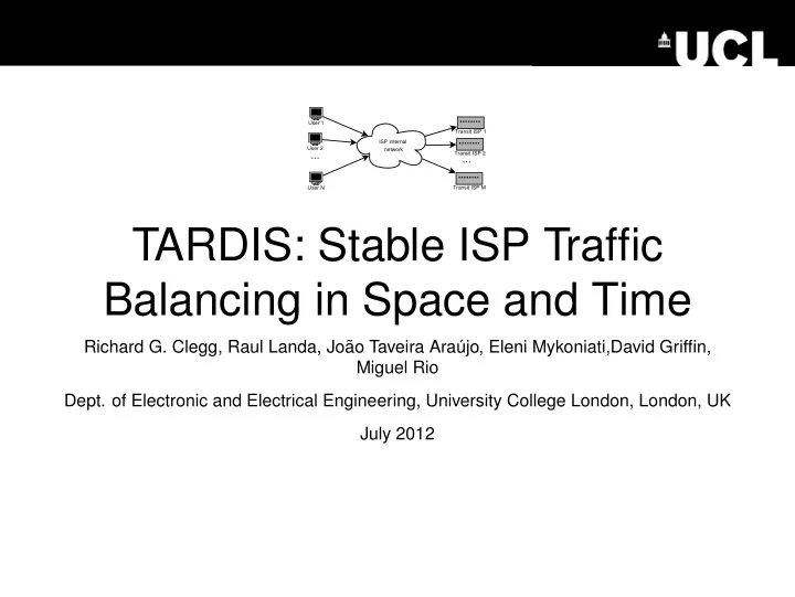
TARDIS: Stable ISP Traffic Balancing in Space and Time Richard G. - PowerPoint PPT Presentation

User 1 Transit ISP 1 ISP internal User 2 network ... Transit ISP 2 ... User N Transit ISP M TARDIS: Stable ISP Traffic Balancing in Space and Time Richard G. Clegg, Raul Landa, Jo˜ ao Taveira Ara´ ujo, Eleni Mykoniati,David Griffin, Miguel Rio Dept. of Electronic and Electrical Engineering, University College London, London, UK July 2012

Introduction Problem statement (vague) Given an eyeball ISP with a number of possible exits to its network (with different billing schemes) and applications which have some flexibility to move their traffic, how should the ISP direct the application to reduce its bill? The system should allow: • Traffic to be shifted in space – moved to different transit or local links to reduce costs. • Traffic to be shifted in time – delayed by several hours (under the user/application’s control) to reduce cost. • The costs must be set at correct values and the resulting traffic shifts must take place in a stable manner.

Simplified system diagram User 1 Transit ISP 1 ISP internal User 2 network ... Transit ISP 2 ... User N Transit ISP M N users send traffic to M transit links (note that link may be a proxy for different billing schemes on same link or it may represent a local link with zero or fixed monthly cost).

Shifting traffic in time and space Time shifting of traffic Allow users to delay traffic (for example to overnight) in order to smooth ISP traffic patterns and reduce the 95th percentile bill. Existing research includes “Good things come to those who (can) wait”, “Time-Dependent Internet pricing” and others. Space shifting of traffic Allows traffic to be diverted to other destinations to reduce ISP transit costs. Existing research includes ALTO/P4P , ONO “Taming the torrent: a practical approach to reducing cross-ISP traffic in peer-to-peer systems”, “Content aware traffic engineering” and many others.

The solution: TARDIS TARDIS: Traffic Assignment and Retiming Dynamics with Inherrent Stability (moves traffic in time and space).

95th percentile billing – an opportunity Traffic level Time of day • Split total traffic in billing period T into smaller periods t with traffic f 1 , f 2 , . . . . • Discard the 5% highest f i and choose the next one – this is f ( 95 ) . The total charge is $ pf ( 95 ) where p is the stated rate. • Clearly there is a gain to be made by moving traffic in time (and space) but how should this be done?

Aside – what traffic can swap and how? • Space swap: Traffic to CDNs and large providers is at multiple locations. (“Content Aware traffic engineering” estimates this is 40% of all traffic). ISPs could transparently change the used CDN node. • Space swap: P2P systems contribute a respectable proportion of traffic. If users were willing to install the software interfaces like CINA and ALTO could inform them which peers to choose. • Space swap: Click hosts have a large traffic share hosted in several networks. ISPs could transparently reroute or users could install software which selected the best. • Time swap: ISPs could retime transfers between CDN nodes and data centers (they probably do this already). • Time swap: Users could be incentivised to delay long downloads to overnight (Internet Post Office).

Problem statement (more specific) Pricing problem Given several links and existing traffic profiles for them, how can an effective price for each slot be created which reflects the pricing scheme and traffic profile. Assingment problem Given prices for each slot, reassign traffic (in a way compatible with user ability to choose between slots) to reduce prices.

The pricing solution: Shapley gradient • The Shapley value is a commonly used notion in game theory. • It formalises the notion of assessing a single user’s contribution to a non-additive score. • Here we adapt this to the Shapley gradient. • This assesses the change to price a user makes by adding traffic in a single slot. • It allows a comparison between different pricing schemes at different times. • Works for schemes other than “linear” and “95th percentile”.

Solving the assignment problem • It is often thought that setting a price “solves” the problem. • Here though, prices alone are not sufficiently informative. • It may be that two “slots” are only equally priced with an unequal traffic split. • The road traffic concept of Wardrop equilibrium is used as a target for assigment. • We use the concept of traffic splits within “choice sets”. • A dynamical system based upon adjusting splits is created. • This is shown to be Lyapunov stable under modest assumptions.

Data used Japanese data set Data is from MAWI data set. It is derived from full non anonymous IP packets. 10,000 users (inside network). Only a three continuous days of data available. Start and end IP addresses known. No prices for links known. European data set Data is from a European ISP . 40,000 users and seven full days of traffic. No mapping to the outgoing transit links (or knowledge of the nature of these links). No prices for links known.

Test framework (diagram)

Modelling assumptions • Need to assume how traffic originally maps to egresses. • Need to assume a proportion of users who can-and-will time swap and who can-and-will space swap – for modelling simplicity willingness and ability are rolled into a single variable. • Need to assume how users will respond to “split percentages” (all or nothing vs proportional) • Need to define prices on links – try HIGH variation (25:5:1) LOW variation (4:2:1) EQUAL prices (1:1:1). • Need to define maximum delay for time swap (12 hours, 18 hours, 24 hours).

EU space but no time swapping 1.2 20% link swappers 40% link swappers 60% link swappers Day cost as proportion of first day 1.1 80% link swappers 100% link swappers 1 0.9 0.8 0.7 0.6 0 10 20 30 40 50 60 70 80 90 100 Time (days)

MAWI data, space but no time swapping 1.2 20% link swappers Day cost as proportion of first iteration cost 40% link swappers 1.1 60% link swappers 80% link swappers 100% link swappers 1 0.9 0.8 0.7 0.6 0.5 0.4 0 10 20 30 40 50 60 70 80 90 100 Time (days)

EU data, time but no space swapping 1 20% time swappers (smoothed) 40% time swappers (smoothed) 60% time swappers (smoothed) 0.95 Day cost as proportion of first day 80% time swappers (smoothed) 0.9 0.85 0.8 0.75 0.7 0.65 0 10 20 30 40 50 60 70 80 90 100 Time (days)

MAWI data, time but no space swapping 1 20% time swappers (smoothed) Day cost as proportion of first iteration cost 40% time swappers (smoothed) 0.95 60% time swappers (smoothed) 80% time swappers (smoothed) 0.9 0.85 0.8 0.75 0.7 0.65 0.6 0.55 0 10 20 30 40 50 60 70 80 90 100 Time (days)

EU data, space and time swapping 1 Time swappers 0% Final cost (as proportion of no swap cost) Time swappers 20% Time swappers 40% 0.9 Time swappers 60% 0.8 0.7 0.6 0.5 0.4 0 20 40 60 80 100 Link swap percentage

Conclusions • TARDIS: Traffic Assignment and Retiming Dynamics with Inherrent Stability – mathematically sound and works well in simulation under a variety of assumptions. • The system is designed for 95th percentile pricing and linear pricing. Could be extended to flat fee and bandwidth cap. • In tests the system produces a stable reassignment of traffic which reduces prices in a wide variety of circumstances. • Link and time swapping can produce large reductions in ISP transit bills. • The degree of reduction depends on the exact nature of the scheme but for many situations a good proportion of the maximum possible benefit can be extracted.

Aside – pricing in the wild • 95th percentile still appears to be dominant for transit. • Increasingly ISPs route traffic through IXPs which have various pricing models (flat rate with bandwidth cap is common). This can be incorporated in our model. • Transit ISPs sometimes unbundle traffic by destination and charge ISPs different rates according to the destination of the traffic (e.g. national less than international). • IXPs often have “stepped” pricing where managers choose a connection size (e.g. 5x1GB links each charged a flat price per month). Our model could not handle this but could handle keeping traffic below a given utilisation for the link capacity chosen.

MAWI data geographical split (incoming) 30 Japan/China inbound US inbound Other destinations inbound 25 Traffic GBytes/hour 20 15 10 5 0 0 10 20 30 40 50 60 70 80 Time (hours)

EU data peak split 2 hours (incoming) 60 Inbound link 1 Inbound link 2 Inbound link 3 50 Traffic GBytes/hour 40 30 20 10 0 0 20 40 60 80 100 120 140 160 180 Time (hours)

MAWI data, space and time swapping 1 Time swappers 0% Final cost (as proportion of no swap cost) Time swappers 20% Time swappers 40% 0.9 Time swappers 60% 0.8 0.7 0.6 0.5 0.4 0.3 0 20 40 60 80 100 Link swap percentage

EU data: Changing the price variance (1:1:1) (1:2:4) (1:5:25) 1.4 40% link swappers (high cost variance) Day cost as proportion of first iteration cost 40% link swappers (low cost variance) 40% link swappers (equal costs) 1.2 80% link swappers (high variance) 80% link swappers (low variance) 80% link swappers (equal costs) 1 0.8 0.6 0.4 0.2 0 10 20 30 40 50 60 70 80 90 100 Time (days)