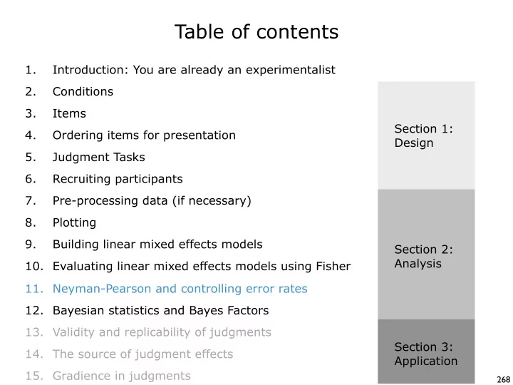
Table of contents 1. Introduction: You are already an - - PowerPoint PPT Presentation

Table of contents

268

Conditions Items Ordering items for presentation Judgment Tasks Recruiting participants Pre-processing data (if necessary) Introduction: You are already an experimentalist 1. 2. 3. 4. 5. 6. 7. Plotting 8. Building linear mixed effects models 9. Evaluating linear mixed effects models using Fisher 10. Bayesian statistics and Bayes Factors 12. Validity and replicability of judgments 13. The source of judgment effects 14. Gradience in judgments 15. Section 1: Design Section 2: Analysis Section 3: Application Neyman-Pearson and controlling error rates 11.

Going further: Neyman-Pearson NHST

269

Jerzy Neyman (1894-1981) Ego Pearson (1895-1980) Neyman and Pearson were fans

• f Fisher’s work, but they

thought there was a logical problem with his approach. While it is all well and good to say that the p-value is a measure of strength of evidence against the null hypothesis, at some point you have to make a decision to reject the null hypothesis, or not. Fisher himself had suggested that p<.05 was a good criterion for deciding whether to reject the null hypothesis or not. Neyman and Pearson decided to take this one step further, and really work out what it would mean to base a statistical theory on the idea of decisions to reject the null hypothesis.

Going further: Neyman-Pearson NHST

270

There are two states of the world: the null hypothesis is either true or false. Tenet 1: You can never know if the null hypothesis is true or false. Tenet 2: This actually follows from the philosophy of science and the problem of induction. In the absence of certainty about the state of the world, all you can do is make a decision about how to proceed based on the results of your

• experiment. You can choose to reject the null hypothesis, or you can choose

not to reject the null hypothesis. This sets up four possibilities: two states of the world and two decisions that you could make. Type I Error Correct Action Correct Action Type II Error State of the World Decision H0 True H0 False Reject H0 Accept H0

Going further: Neyman-Pearson NHST

271

Type I Error Correct Action Correct Action Type II Error State of the World Decision H0 True H0 False Reject H0 Accept H0 This is when the null hypothesis is true, but you mistakenly reject it. Type I Error: This is when the null hypothesis is false, but you mistakenly fail to reject it. Type II Error: Take a moment to really think about what these two errors are. What do you think about the relative importance of each one?

Going further: Neyman-Pearson NHST

272

Neyman-Pearson, and many others, have suggested that Type I errors are more damaging than Type II errors. The basic idea is that science is focused on rejecting the null hypothesis, not accepting it. (To publish a paper, you have to reject the null hypothesis.) So a Type I error would mean making a decision (or publishing a result) that misleads science. Type II errors are also important, but not equally so. Failing to reject the null hypothesis is simply a failure to advance science. It doesn’t (necessarily) mislead the way that a Type I error does. Type I Error Correct Action Correct Action Type II Error State of the World Decision H0 True H0 False Reject H0 Accept H0

Going further: Neyman-Pearson NHST

273

This is when the null hypothesis is true, but you mistakenly reject it. Type I Error: If you accept the importance of Type I errors, then you will want to keep the rate of Type I errors as low as possible. Under the Neyman-Pearson approach, which emphasizes the decision aspect of science, you can control your Type I error rate by always using the same criterion for your decisions. alpha level / alpha criterion: This is the criterion that you use to make your decision. By keeping it constant, you keep the number of Type I errors that you will make constant too. For example, if you set your alpha level to .05, then you only decide to reject the null hypothesis if your p-value is less than .05. Similarly, if you set your alpha level to .01, then you only decide to reject the null hypothesis if your p-value is less than .01. Take a moment to think about how setting an alpha level will control your Type I error rate.

Going further: Neyman-Pearson NHST

274

There is an important relationship between your alpha level and the number of Type I errors that you will make: If you apply the same alpha level consistently over the long-run, your Type I error rate will be less than or equal to your alpha level. Here’s a thought experiment:

• 1. Imagine that the null hypothesis is TRUE.
• 2. Now, imagine that you run an experiment and derive a test statistic.
• 3. Next, imagine that you run a second experiment and derive a test statistic.
• 4. And then, imagine that you ran the experiment 10,000 times…
• 5. This should be familiar. You just derived a reference distribution of the test

statistic under the null hypothesis!

• 6. Now ask yourself, if your alpha level is .05, how often will you derive a p-

value less than .05? In short, how often would you make a Type I Error? We can run this in R. There is code for it in alpha.demonstration.r.

Going further: Neyman-Pearson NHST

275

It is important to understand the relationship between these concepts: This is when the null hypothesis is true, but you mistakenly reject it. Type I Error: The probability of obtaining a test statistic equal to, or more extreme than, the one you observed under the null hypothesis. p-value: α-level: The threshold below which you decide to reject the null hypothesis If you consistently base your decisions on the alpha level, then your Type I error rate will either be less than or equal to your alpha level! We say that it might be less because we admit that the null hypothesis might be false for some experiments. Every time the null hypothesis is false, you make one less Type I Error, so the rate goes down a bit!

Multiple comparisons

Multiple comparisons

277

When people say “multiple comparisons”, what they mean is running more than one statistical test on a set of experimental data. The simplest design where this will arise is a one-factor design with three

• levels. Maybe something like this:

What do you think that John bought? What do you wonder whether John bought? What do you wonder who bought? An F-test (ANOVA) or linear mixed effects model

• n this design will ask the following question:

What is the probability of the data under the assumption that the three means are equal? null hypothesis How many patterns of results will yield a low p-value under this null hypothesis?

A significant result tells us relatively little

278

Here are all (I think?) of the patterns of results that will yield a significant result in a one-way / three-level test. As you can see, a significant result doesn’t tell us very much. If we want to know which of these patterns is the one in our data, we need to compare each level to every other level one pair at a time: = and and test test test

The multiple comparison problem

Review: Neyman-Pearson NHST

280

Type I Error Correct Action Correct Action Type II Error State of the World Decision H0 True H0 False Reject H0 Accept H0 This is when the null hypothesis is true, but you mistakenly reject it. Type I Error: This is when the null hypothesis is false, but you mistakenly fail to reject it. Type II Error: α-level: The threshold at which you decide to reject the null hypothesis.

Review: Neyman-Pearson NHST

281

• 6
• 3

Review: the alpha level

282

Here is how the alpha level works: Imagine that the null hypothesis is true for your phenomenon. 1. And let’s run an experiment testing this difference 10,000 times, saving the statistic each time. 2. real world distribution of stats The result will be a distribution of real- world test statistics, obtained from experiments where the null hypothesis is true. 3.

• 6
• 3

• 6
• 3

real world distribution But also notice that this distribution will be nearly identical to the hypothetical null distribution for your test statistic (because the null hypothesis was true in the real world). This will be important later. 4.

• 6
• 3

null distribution =

• 6
• 3

Review: the alpha level

283

Now let’s choose a threshold to cut the distribution into two decisions: non- significant and significant 5. null distribution Remember we call this the alpha level. alpha level reject the null accept the null Also remember that this is a criterion chosen based on the null distribution (because this is a null hypothesis test).

• 6
• 3

Now we apply this threshold to each of our 10,000 experiments, one at a time as we run them. 6. real world experiments So for each experiment, we can label it as a correct decision (accept the null) or a false positive (reject the null). dividing line false positives correct decisions And to make life easier, we can visualize this as a distribution of results, with a dividing line between the two types.

• 6
• 3

Review: the alpha level

284

Now here is the final question. How many false positives happened in our 10,000 experiments? 7. null distribution We could count them. But what I want to show you is the consequence of the identity that happened back in step 4. alpha level reject the null accept the null

• 6
• 3

real world experiments dividing line false positives correct decisions

• 6
• 3

real world distribution

• 6
• 3

null distribution = Because our real world distribution is identical to the null distribution (the null hypothesis is true), our alpha level is identical to the dividing line between correct decisions and false positives: = In this way, the alpha level is the maximum type I error rate (because the maximum number of errors occurs when the null is true).

There are different alphas

285

The probability that an experiment contains at least one Type I error. We can call this rate αEW. Experimentwise Error Rate: Familywise Error Rate: This is just like experimentwise error, but allows you to define sub-groups of comparisons inside of an experiment called a “family”. So this is the probability that a family contains at least one error. In most experiments, there is just one family, so this will be equal to the experimentwise error rate. Per Comparison Error Rate: The probability that any one comparison is a Type I error (number of errors/number of comparisons). You set this by choosing a threshold for your decisions. We can call both the threshold and the resulting error rate αPC. number of statistical tests αPC = number of errors number of experiments αEW = number of experiments with 1 or more errors

Visualizing the different alphas

286

e1 e2 e3 e20 . . . comp1 comp2 comp3 number of statistical tests αPC = number of errors Imagine your experiment has 3 comparisons, and you run that experiment 20

• times. Let’s say you set αPC to .05. Here are your results:

60 αPC = 3 = .05 number of experiments αEW = number of experiments w/errors 20 αEW = 3 = .15 When you make multiple comparisons, αEW is larger than αPC. This is the multiple comparisons problem!

An equation for relating αEW to αPC

287

The relationship between αPC n αEW is lawful, and follows this equation αEW = 1 - (1-αPC)C where C is the number of comparisons. So for 3 comparisons and an αPC set to .05, the maximum αEW will be: αEW = 1 - (1-.05)3 αEW = .142625 There is code in multiple.comparisons.r to demonstrate αEW,and how the αEW will always be more than αPC. e1 e2 e3 e20 . . . comp1 comp2 comp3 The take-home message is that multiple comparisons increases your type I error rate for the entire experiment!

Controlling Experimentwise Error (or Familywise Error) with the Bonferroni Correction

Controlling EW/FW error

289

So now you can see that setting an alpha level of .05 for each comparison only controls error at the comparison level. If you want to control errors at the experiment (or family) level, you need to make an adjustment to your decision criterion. Luckily, the equation for EW/FW error tells us exactly how to do that: αEW = 1 - (1-αPC)C Since EW/FW error is dependent on αPC, all we have to do is choose an αPC that gives us the αEW that we want! You could do this through guessing-and-testing if you want, but Olive Dunn figured out a much faster way using one of Carlo Bonferroni’s inequalities: X ≥ 1 - (1-(X/C))C As you can see, this inequality looks very similar to the αEW equation above…

The Bonferroni Correction (by Olive Dunn)

290

Here is how you can use Bonferroni’s inequality to set your maximum αEW: X ≥ 1 - (1-(X/C))C αEW = 1 - (1-αPC)C αEW ≥ 1 - (1-(αEW/C))C First, replace the X with αEW because that is what we care about. (And C is the number of comparisons). Next, notice that the term αEW/C is in the position that αPC occupies in the αEW equation. From that, it follows that if we set αPC to αEW/C we can keep our αEW at or below the number we want! αPC αEW C = The Bonferroni correction (by Olive Dunn) states that we can control our experimentwise error rate (αEW) by setting our decision threshold per comparison (αPC) to our intended experimentwise error rate divided by the number of comparisons (αEW/C). See multiple.comparisons.r for a demo!

Why does αPC/C eliminate errors?

291

To see why the Bonferroni correction eliminates errors (over the long run!), all you need to do is think about the distribution of p-values. αPC The original αPC divides the distribution of p-values into those that lead to acceptance of H0, and those that lead to an error (rejection of H0) If you have two comparisons per experiment, you will basically double the number of errors over the long run. These errors will be evenly distributed throughout the error zone in the tail. The Bonferroni correction cuts the tail. In this case, it cuts it in

• half. This means that you will

eliminate half of the errors, which is what you want! αPC/2 The same logic scales up to any number of comparisons. By cutting the zone, on average, you will move C-1 errors into the non-error zone!

Planned versus Post-Hoc Comparisons

Two types of comparisons

293

This is a comparison that you specify before running your experiment (and crucially before looking at any data). Basically, you have a specific hypothesis, and decide that the best way to test it is to compare certain levels to each other. Planned Comparison: This is a comparison that you decide to run after looking at your data. Basically, you see a difference in your data, and are curious to know if it is significant. This isn’t theory-driven testing, this is data-driven testing. Post-hoc Comparison: I know it sounds strange, but under NHST, this difference matters for the probabilities of Type I errors.

Planned Comparisons are safe

294

Everything that we’ve said so far about the Bonferroni correction holds for planned comparisons. Theory-driven comparisons are safe! As a concrete example, let’s say that there are 3 possible comparisons in your experiment. That means there are a maximum of 3 comparisons per hypothetical replication. e1 e2 e3 e20 . . . comp1 comp2 comp3

Planned Comparisons are safe

295

Everything that we’ve said so far about the Bonferroni correction holds for planned comparisons. Theory-driven comparisons are safe! As a concrete example, let’s say that there are 3 possible comparisons in your experiment. That means there are a maximum of 3 comparisons per hypothetical replication. e1 e2 e3 e20 . . . comp1 comp2 comp3 Now, let’s say that you decide before you see the data that you are only going to look at comparison 1 and comparison 2. That eliminates, over the long run, one third of the errors. By setting αPC to .05/2 = .025, you will eliminate half of the remaining errors

• ver the long run.

And the end result is, over the long run, 1 error out of 20 experiments!

Post-hoc Comparisons are not safe!

296

Let’s say you look for the biggest difference in each experiment (out of the 3), and test that one with an alpha level of .05. What is your EW error rate? This looks like a single comparison experiment because you are only running one test, so C=1. But you are running the largest difference you see. e1 e2 e3 e20 . . . comp1 comp2 comp3 So, you only ran 20 comparisons, but you end up with 3 errors for an error rate of .15! This means that all of the errors will be in your tests (because they are large by definition). The problem is that you eliminated 2 comparisons (so C=1) but you didn’t eliminate any of the errors. So you didn’t get the benefit of eliminating comparisons.

OK, so what do we do?

297

If you have planned comparisons, just run the Bonferroni correction with your actual number of comparisons (C). If you have post-hoc comparisons, you can’t use the actual number of comparisons, because you chose them using the data. The only downside of this option is that this could be a very extreme correction (imagine 10 possible comparisons, which would be .05/10=.005). If the number of comparisons you are actually running is small, and the number of possible comparisons is large, you may be over-correcting, and thus making it less likely that you will detect significant differences that are really there. Run the Bonferroni correction with C equal to the maximum number of comparisons licensed by your experimental design. Option 1: Run one of the methods that have been proposed to replace the Bonferroni method, like Tukey’s Honestly Significant Difference (Tukey’s HSD) or Scheffe’s method. These were designed to provide good control of αEW without sacrificing as much power as the Bonferroni method. Option 2:

Criticisms of NHST

298 Balluerka, N., Goméz, J., & Hidalgo, D. (2005). The controversy over null hypothesis significance testing revisited. Methodology, 1(2), 55-70. Cohen, J. (1994). The earth is round (p < .05). American Psychologist, 49, 997-1003. Gigerenzer, G. (2004). Mindless statistics. The Journal of Socio-Economics, 33, 587-606. Hubbard, R., & Lindsay, R. M. (2008). Why p values are not a useful measure of evidence in statistical significance testing. Theory and Psychology 18(1), 69-88. Nickerson, R. (2000). Null hypothesis significance testing: A review of an old and continuing

• controversy. Psychological Methods, 5(2), 241-301

Hubbard, R & M. J. Bayarri. (2003) P Values are not Error Probabilities.

Despite the ubiquity of NHST as the analysis method for psychology, most people who think seriously about data analysis are critical of it. I would love to spend a couple of weeks talking about these criticisms and really diving into the heart of the data analysis problem. But there is not time. But you all should know enough now to read papers that are critical of NHST and think about the problems for yourself. So I’ve collected a bunch of good

• nes into folder you can download from the website. They are: