Survival analysis in R Niels Richard Hansen This note describes a - PDF document

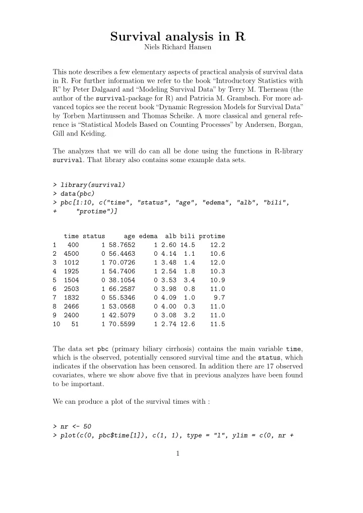
Survival analysis in R Niels Richard Hansen This note describes a few elementary aspects of practical analysis of survival data in R. For further information we refer to the book “Introductory Statistics with R” by Peter Dalgaard and “Modeling Survival Data” by Terry M. Therneau (the author of the survival -package for R) and Patricia M. Grambsch. For more ad- vanced topics see the recent book“Dynamic Regression Models for Survival Data” by Torben Martinussen and Thomas Scheike. A more classical and general refe- rence is “Statistical Models Based on Counting Processes” by Andersen, Borgan, Gill and Keiding. The analyzes that we will do can all be done using the functions in R-library survival . That library also contains some example data sets. > library(survival) > data(pbc) > pbc[1:10, c("time", "status", "age", "edema", "alb", "bili", + "protime")] time status age edema alb bili protime 1 400 1 58.7652 1 2.60 14.5 12.2 2 4500 0 56.4463 0 4.14 1.1 10.6 3 1012 1 70.0726 1 3.48 1.4 12.0 4 1925 1 54.7406 1 2.54 1.8 10.3 5 1504 0 38.1054 0 3.53 3.4 10.9 6 2503 1 66.2587 0 3.98 0.8 11.0 7 1832 0 55.5346 0 4.09 1.0 9.7 8 2466 1 53.0568 0 4.00 0.3 11.0 9 2400 1 42.5079 0 3.08 3.2 11.0 10 51 1 70.5599 1 2.74 12.6 11.5 The data set pbc (primary biliary cirrhosis) contains the main variable time , which is the observed, potentially censored survival time and the status , which indicates if the observation has been censored. In addition there are 17 observed covariates, where we show above five that in previous analyzes have been found to be important. We can produce a plot of the survival times with : > nr <- 50 > plot(c(0, pbc$time[1]), c(1, 1), type = "l", ylim = c(0, nr + 1

+ 1), xlim = c(0, max(pbc$time[1:nr]) + 10), ylab = "nr", xlab = "Survival tim > for (i in 2:nr) lines(c(0, pbc$time[i]), c(i, i)) > for (i in 1:nr) { + if (pbc$status[i] == 0) + points(pbc$time[i], i, col = "red", pch = 20) + if (pbc$status[i] == 1) + points(pbc$time[i], i) + } 50 ● ● ● ● ● ● ● ● ● ● 40 ● ● ● ● ● ● ● ● ● ● 30 ● ● ● ● ● nr ● ● ● ● 20 ● ● ● ● ● ● ● ● ● ● ● 10 ● ● ● ● ● ● ● ● ● ● 0 0 1000 2000 3000 4000 Survival time Estimation of the survival function using the Kaplan-Meier estimator can be done using the survfit function. > pbc.surv <- survfit(Surv(time, status), data = pbc) > pbc.surv Call: survfit(formula = Surv(time, status), data = pbc) n events median 0.95LCL 0.95UCL 418 161 3395 3090 3853 2

> plot(pbc.surv, mark.time = FALSE) 1.0 0.8 0.6 0.4 0.2 0.0 0 1000 2000 3000 4000 The result from survfit is an R object of type survfit . Taking summary of a survfit object provides the non-parametric estimate of the survival function including additional information as a long list. The plot with the added, pointwise confidence bands is perhaps more informative. Setting mark.time=FALSE prevents all the censored observations to be marked on the plot by a “+”. The function Surv applied to the time and status variables for the PBC data is a function that create a survival object. A major point in a data set like the PBC data above is that we record covariate information on the individuals. It is no problem to split the estimation of the survival function according to a factor such as the binary edema variable in the PBC data. > pbc.surv <- survfit(Surv(time, status) ~ edema, data = pbc) > plot(pbc.surv, conf.int = TRUE, col = c("red", "blue")) 3

1.0 0.8 0.6 0.4 0.2 0.0 0 1000 2000 3000 4000 From the plot it seems clear that individuals without edema have a larger chance of a large survival time than those with edema. This can also be tested formally with the so-called log-rank test. > survdiff(Surv(time, status) ~ edema, data = pbc) Call: survdiff(formula = Surv(time, status) ~ edema, data = pbc) N Observed Expected (O-E)^2/E (O-E)^2/V edema=0 368 121 151.0 5.94 96 edema=1 50 40 10.0 89.28 96 Chisq= 96 on 1 degrees of freedom, p= 0 But what about including the other covariates also – especially the continuous ones? This can be handled in the framework of the Cox proportional hazards model. > pbc.surv <- coxph(Surv(time, status) ~ edema, data = pbc) > summary(pbc.surv) 4

Call: coxph(formula = Surv(time, status) ~ edema, data = pbc) n= 418 coef exp(coef) se(coef) z p edema 1.63 5.09 0.185 8.82 0 exp(coef) exp(-coef) lower .95 upper .95 edema 5.09 0.197 3.54 7.3 Rsquare= 0.129 (max possible= 0.985 ) Likelihood ratio test= 57.7 on 1 df, p=3e-14 Wald test = 77.7 on 1 df, p=0 Score (logrank) test = 96 on 1 df, p=0 We can tell from the summary that the β corresponding to the covariate edema is significantly different from 0. We also see that the hazard rate for those with edema=1 is estimated as roughly 5 times the base-line hazard rate α 0 ( t ). We can include more covariates. > pbc.surv <- coxph(Surv(time, status) ~ edema + age + alb + bili + + protime, data = pbc) > summary(pbc.surv) Call: coxph(formula = Surv(time, status) ~ edema + age + alb + bili + protime, data = pbc) n= 418 coef exp(coef) se(coef) z p edema 0.7222 2.059 0.20764 3.48 5.1e-04 age 0.0365 1.037 0.00811 4.50 6.8e-06 alb -0.9266 0.396 0.20898 -4.43 9.2e-06 bili 0.1246 1.133 0.01271 9.80 0.0e+00 protime 0.1928 1.213 0.05770 3.34 8.3e-04 exp(coef) exp(-coef) lower .95 upper .95 edema 2.059 0.486 1.371 3.093 age 1.037 0.964 1.021 1.054 alb 0.396 2.526 0.263 0.596 bili 1.133 0.883 1.105 1.161 protime 1.213 0.825 1.083 1.358 5

Rsquare= 0.36 (max possible= 0.985 ) Likelihood ratio test= 186 on 5 df, p=0 Wald test = 218 on 5 df, p=0 Score (logrank) test = 309 on 5 df, p=0 It is of course also possible to transform the covariates before using them in the regression. For example; > pbc.surv <- coxph(Surv(time, status) ~ edema + age + log(bili) + + log(alb) + log(protime), data = pbc) > summary(pbc.surv) Call: coxph(formula = Surv(time, status) ~ edema + age + log(bili) + log(alb) + log(protime), data = pbc) n= 418 coef exp(coef) se(coef) z p edema 0.6613 1.937 0.20595 3.21 1.3e-03 age 0.0382 1.039 0.00768 4.97 6.5e-07 log(bili) 0.8975 2.453 0.08271 10.85 0.0e+00 log(alb) -2.4524 0.086 0.65707 -3.73 1.9e-04 log(protime) 2.3458 10.442 0.77425 3.03 2.4e-03 exp(coef) exp(-coef) lower .95 upper .95 edema 1.937 0.5162 1.2938 2.901 age 1.039 0.9625 1.0234 1.055 log(bili) 2.453 0.4076 2.0863 2.885 log(alb) 0.086 11.6167 0.0237 0.312 log(protime) 10.442 0.0958 2.2895 47.624 Rsquare= 0.429 (max possible= 0.985 ) Likelihood ratio test= 234 on 5 df, p=0 Wald test = 233 on 5 df, p=0 Score (logrank) test = 297 on 5 df, p=0 One will need tools for model diagnostic. One simple idea is as follows. The survival functions, S i ( t ), for different individuals, i , must fulfill that � t 0 α ( s )d s + X T log( − log( S i ( t )) = log i β are parallel. Now we don’t know each individual survival function but if we group individuals with similar covariates we might be able to estimate, non- parametrically, the survival functions for the groups and then visually inspect if the survival functions look parallel. 6

Considering only one variable, bili , we divide into three groups. > group <- 1 * (pbc$bili > 1.1) + 1 * (pbc$bili > 3.3) > cfit <- survfit(Surv(time, status) ~ group, data = pbc) > plot(cfit, mark.time = FALSE, fun = "cloglog", xlim = c(40, 5000)) 1 0 −1 −2 −3 −4 −5 50 100 200 500 1000 2000 Including in addition edema , which is already discrete we get a total of 6 groups. Note the additive specification in the formula below, which in reality stratifies the estimation into all 6 possible combinations. > cfit <- survfit(Surv(time, status) ~ group + edema, data = pbc) > plot(cfit, mark.time = FALSE, fun = "cloglog", xlim = c(40, 5000)) 7

1 0 −1 −2 −3 −4 −5 50 100 200 500 1000 2000 It is left to the reader to judge the plots ... A good question is what happens if more stratification according to other variables is applied. A Theory We consider n individuals, T ∗ 1 , . . . , T ∗ n independent, positive random variables (survival times). Estimation of the distribution by the empirical distribution: n F ( t ) = 1 ˆ � 1( T ∗ i ≤ t ) n i =1 and the survival function S ( t ) = 1 − F ( t ) n F ( t ) = 1 S ( t ) = 1 − ˆ ˆ � 1( T ∗ i > t ) . n i =1 8