Supplement A: Break-even analysis Break even analysis Analysis to - - PDF document

1

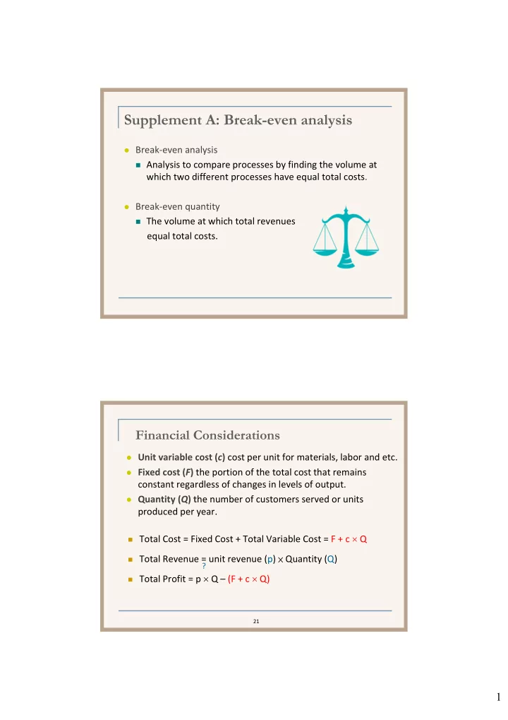
Supplement A: Break-even analysis

 Break‐even analysis  Analysis to compare processes by finding the volume at

which two different processes have equal total costs.

 Break‐even quantity  The volume at which total revenues

equal total costs.

21

Financial Considerations

 Total Cost = Fixed Cost + Total Variable Cost = F + c  Q  Total Revenue = unit revenue (p) × Quantity (Q)  Total Profit = p  Q – (F + c  Q)

?

 Unit variable cost (c) cost per unit for materials, labor and etc.  Fixed cost (F) the portion of the total cost that remains

constant regardless of changes in levels of output.

 Quantity (Q) the number of customers served or units

produced per year.

2

22

Break-Even Analysis

Total Profit = p × Q – (F + c × Q) Total Profit = 0  p × Q = (F + c × Q)

F

c p F 

Break‐even quantity  Q =

Example A.1

A new procedure will be offered at $200 per patient. The fixed cost per year would be $100,000 with variable costs of $100 per patient. What is the break‐even quantity for this service?

Q = F p – c = 1,000 patients = 100,000 200 – 100

Total annual costs Fixed costs Break-even quantity Profit Loss Patients (Q) Dollars (in thousands)

400 – 300 – 200 – 100 – 0 –

| | | |

500 1000 1500 2000 (2000, 300) Total annual revenues (2000, 400)

3

Financial Analysis

 Consider time value of money  Present value=150,000, annual interest rate=5%  Payback period=5 years  Annual net cash flow=

=PMT(5%,5,150000,0) =$34646

24

Evaluating Alternatives

 Fb : The fixed cost (per year) of the buy option  Fm : The fixed cost of the make option 

cb : The variable cost (per unit) of the buy option



cm : The variable cost of the make option

 Total cost to buy = Fb + cbQ  Total cost to make = Fm + cmQ

Fb + cbQ = Fm + cmQ  Q = Fm – Fb cb – cm

4

Example A.3

 A fast‐food restaurant is adding salads to the menu.  Fixed costs are estimated at $12,000 and variable costs

totaling $1.50 per salad.

 Preassembled salads could be purchased from a local

supplier at $2.00 per salad. It would require additional refrigeration with an annual fixed cost of $2,400

 The price to the customer will be the same.  Expected demand is 25,000 salads per year.

Q =Fm – Fb cb – cm = 19,200 salads = 12,000 – 2,400 2.0 – 1.5

Supplement B: Waiting Line Models

Q: What are waiting lines and why do they form? A: Waiting Lines form due to a temporary imbalance between the demand for service and the capacity of the system to provide the service. Customer population Service system

Waiting line Priority rule Service facilities

Served customers

5

Structure of Waiting-Lines

• 1. An input, or customer population, that generates

potential customers

• 2. A waiting line of customers (號碼牌)
• 3. The service facility, consisting of a person (or crew), a

machine (or group of machines), or both necessary to perform the service for the customer

• 4. A priority rule, which selects the next customer to be

served by the service facility

Waiting Line Arrangements

Service facilities Service facilities

Single Line Multiple Lines

6

Service Facility Arrangements

Service facility

Single channel, single phase Single channel, multiple phase

Service facility 1 Service facility 2

Multiple channel, single phase

Service facility 1 Service facility 2 Service facility 3 Service facility 4 Service facility 1 Service facility 2

Multiple channel, multiple phase

Random Arrivals

Poisson arrival distribution

Pn =

for n = 0, 1, 2,…

(T)n n!

Pn =Probability of n arrivals in T time periods  = Average numbers of customer arrivals per period e = 2.7183

e-T

 = 2 customers per hour, T = 1 hour, and n = 4 customers.

P4 =

= = 0.090 16 24 [2(1)]4 4! e–2(1)

e–2

7

Priority Rules

 First‐come, first‐served (FCFS)  Earliest due date (EDD)  Shortest processing time (SPT)  Preemptive discipline

(emergencies first) P(t ≤ T) = 1 – e–T

μ = average number of customer completing service per period t = actual service time of the customer T = target service time

Customer Service Times

Exponential service time distribution  = 3 customers per hour, T = 10 minutes = 0.167 hour. P(t ≤ 0.167 hour) = 1 – e–3(0.167) = 1 – 0.61 = 0.39

8

Waiting-Line Models to Analyze Operations

 Balance costs (capacity, lost sales) against benefits

(customer satisfaction)

 Operating characteristics

• 1. Line length
• 2. Number of customers in system
• 3. Waiting time in line
• 4. Total time in system
• 5. Service facility utilization

Single-Server Model

 Single‐server, single waiting line, and only one phase  Assumptions are:

• 1. Customer population is infinite and patient
• 2. Customers arrive according to a Poisson distribution,

with a mean arrival rate of 

• 3. Service distribution is exponential with a mean

service rate of 

• 4. Mean service rate exceeds mean arrival rate  < 
• 5. Customers are served FCFS
• 6. The length of the waiting line is unlimited

9

 = Average utilization of the system = < 1   L = Average number of customers in the system =   –  Lq = Average number of customers in the waiting line =  L W = Average time spent in the system, including service = 1  –  Wq = Average waiting time in line =  W n = Probability that n customers are in the system = (1– ) n

Single-Server Model Little’s Law

A fundamental law that relates the number of customers in a waiting‐line system to the arrival rate and average time in system Average time in the system W = L customers  customer/hour Work‐in‐process L = W  = arrival rate

10

Multiple-Server Model



Service system has only one phase, multiple‐channels



Assumptions (in addition to single‐server model)



There are s identical servers



Exponential service distribution with mean 1/



s should always exceed 