Summary Talk based on: The Standard Model in Noncommutative - - PowerPoint PPT Presentation

SLIDE 1

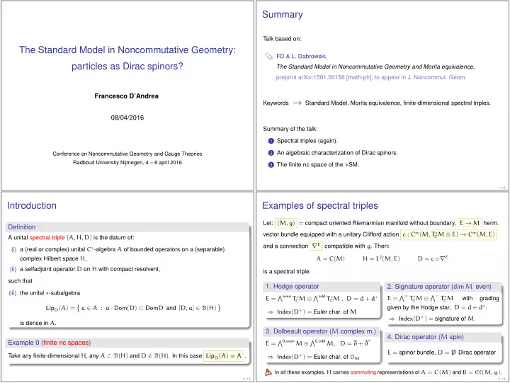
The Standard Model in Noncommutative Geometry: particles as Dirac spinors?

Francesco D’Andrea 08/04/2016

Conference on Noncommutative Geometry and Gauge Theories Radboud University Nijmegen, 4 – 8 april 2016

Summary

Talk based on: FD & L. Dabrowski, The Standard Model in Noncommutative Geometry and Morita equivalence, preprint arXiv:1501.00156 [math-ph]; to appear in J. Noncommut. Geom. Keywords → Standard Model, Morita equivalence, finite-dimensional spectral triples. Summary of the talk:

1 Spectral triples (again). 2 An algebraic characterization of Dirac spinors. 3 The finite nc space of the νSM.

1 / 13

Introduction

Definition

A unital spectral triple (A, H, D) is the datum of: (i) a (real or complex) unital C∗-algebra A of bounded operators on a (separable) complex Hilbert space H, (ii) a selfadjoint operator D on H with compact resolvent, such that (iii) the unital ∗-subalgebra LipD(A) =

• a ∈ A : a · Dom(D) ⊂ DomD and [D, a] ∈ B(H)
• is dense in A.

Example 0 (finite nc spaces)

Take any finite-dimensional H, any A ⊂ B(H) and D ∈ B(H). In this case LipD(A) ≡ A .

2 / 13

Examples of spectral triples

Let: (M, g) = compact oriented Riemannian manifold without boundary, E → M herm. vector bundle equipped with a unitary Clifford action c : C∞(M, T ∗

CM ⊗ E) → C∞(M, E)

and a connection ∇E compatible with g. Then: A = C(M) H = L2(M, E) D = c ◦ ∇E is a spectral triple.

• 1. Hodge operator

E = even T ∗

CM ⊕ odd T ∗ CM , D = d + d∗

⇒ Index(D+) = Euler char. of M

• 2. Signature operator (dim M even)

E = + T ∗

CM ⊕ − T ∗ CM

with grading given by the Hodge star, D = d + d∗. ⇒ Index(D+) = signature of M

• 3. Dolbeault operator (M complex m.)

E = 0,even M ⊕ 0,odd M, D = ∂ + ∂

∗

⇒ Index(D+) = Euler char. of OM

• 4. Dirac operator (M spin)

E = spinor bundle, D = D

/ Dirac operator

In all these examples, H carries commuting representations of A = C(M) and B = Cℓ(M, g).

3 / 13

SLIDE 2

• 5. The Standard Model spectral triple

The underlying geometry is

M × F

(spin manifold) (finite nc space)

with finite-dim. spectral triple (AF, HF, DF, γF, JF) given by:

◮ HF ≃ C32n internal degrees of freedom of the elementary fermions. Total nr:

2 × 4 × 2 × 2 × n = 32n

(weak isospin) (lepton + quark (L,R chirality) (particle or (generations) in 3 colors) antiparticle)

◮ γF = chirality operator ◮ AF = C ⊕ H ⊕ M3(C)

JF = charge conjugation

• gauge group ≈ U(1) × SU(2) × SU(3)

◮ DF encodes the free parameters of the theory.

4 / 13

Algebraic characterization of Dirac spinors

Definition

A unital spectral triple (A, H, D) is called:

◮ even if ∃ γ = γ∗ on H s.t. γ2 = 1, γD = −Dγ and [γ, a] = 0 ∀ a ∈ A; ◮ real if ∃ an antilinear isometry J on H s.t. J2 = ±1, JD = ±DJ, Jγ = ±γJ and ∀ a, b ∈ A:

[a, JbJ−1] = 0

(reality)

[[D, a], JbJ−1] = 0

(1st order)

Theorem

• 1. A closed oriented Riem. manifold M admits a spinc structure iff ∃ a Morita equivalence

C(M)-Cℓ(M, g) bimodule Σ, with Cℓ(M, g) the algebra of sections of the Clifford bundle.

• 2. Σ = C0 sections of the spinor bundle S → M (Dirac spinors in the conventional sense).

Once we have S, we can canonically introduce the Dirac operator D of the spinc structure:

• 3. M is a spin manifold iff ∃ a real structure J on L2(M, S).

5 / 13

What is a noncommutative spin manifold?

For simplicity, let us focus on finite-dimensional spectral triples. ( ⇒ A ≡ LipD(A) and we can use the ring-theoretic Morita equivalence.)

Definition (1-forms)

If (A, H, D) is a spectral triple, we define Ω1

D ⊆ B(H) as:

Ω1

D := Span

• a[D, b] : a, b ∈ A
• Definition (Clifford algebra)

[≈ Lord, Rennie & V´ arilly, J.Geom.Phys. 2012]

We call CℓD(A) ⊆ B(H) the algebra generated by A, Ω1

D and possibly γ (in the even case).

Let A◦ :=

• Ja∗J−1 : a ∈ A
• . The reality and 1st order cond. are equivalent to the statement

A◦ ⊆ CℓD(A)′ :=

• b ∈ B(H) : [b, ξ] = 0 ∀ ξ ∈ CℓD(A)
• .

(⋆)

Definition (Dirac condition)

Elements of H are “Dirac spinors” if (⋆) is an equality: A◦ = CℓD(A)′.

6 / 13

On a property of “Hodge spinors”

In the geometric examples (slide 3), [D, f] = c(df). In the Hodge example: H = Ω•(M)

L2

≃ Cℓ(M, g)

L2

B := CℓD(A) = Cℓ(M, g) Representation of B: by Clifford multiplication on Ω•(M), or by left multiplication on itself. Real structure: J(ω) = ω∗ . The algebra B◦ = JBJ−1 acts by right multiplication on H, that up to completion is a self-Morita equivalence B-bimodule.

Definition (2nd order condition)

(A, H, D, J) satisfies the 2nd order condition if CℓD(A)◦ := J CℓD(A) J−1 ⊆ CℓD(A)′ (⋆⋆)

Remark: this is the old “order-two” condition by Boyle and Farnsworth (cf. also Besnard, Bizi, Brouder).

Definition (Hodge condition)

(dim H < ∞) Elements of H are “Hodge spinors” if (⋆⋆) is an equality: CℓD(A)◦ = CℓD(A)′.

7 / 13

SLIDE 3

Spin + 2nd order

Observation 1.

Dirac condition + 2nd order condition ⇒ Hodge condition. In fact: CℓD(A)◦ ⊆ CℓD(A)′ = A◦ = ⇒ CℓD(A) = A Therefore:

Observation 2.

Dirac condition + 2nd order ⇒ H is a self-Morita equivalence A-bimodule (a “line bundle”). An example of spectral triple satisfying both conditions (Einstein-Yang Mills): A = MN(C) H = A J(a) = a∗ D = 0

8 / 13

Back to the Standard Model. . .

Recall that in the ncg approach to the Standard Model,one has:

M × F

(spin manifold) (finite nc space)

For the continuous part, elements of HM are Dirac spinors. What about the finite part? We have the following dictionary: Geometry ← → Algebra Spinc A-CℓD(A) Morita equivalence Spin A-CℓD(A) Morita equivalence with J Hodge CℓD(A) self-Morita equivalence∗

∗ in progress with L. Dabrowski & A. Sitarz

What kind of nc space is F ?

9 / 13

Postdictions on DF

Not every DF is allowed! ⇒ Restrictions on the free parameters/on the interactions. Constraints of the 1st kind:

1 The parity (γFDF = −DFγF) and 1st (or 2nd) order condition put constraints on DF:

some matrix entries must be zero. For example, the 1st order cond. does not allow a vertex

? e− e−

Nothing forbids taking DF = 0 (all conditions are satisfied). Constraints of the 2nd kind:

2 The request that elements of HF are Dirac spinors (or Hodge spinors) on F implies, in

general, that some matrix entries cannot be zero.

10 / 13

The 1st order condition

Let (A, H, J) be finite dim. One can completely characterize D’s of 1st order:

Theorem ( ≈ Krajewski)

• D ∈ EndC(H) satisfies the 1st order condition iff it is of the form

D = D0 + D1 (†) with D0 ∈ (A◦)′ and D1 ∈ A′.

• D selfadjoint resp. odd ⇒ one can always choose D0 and D1 selfadjoint resp. odd.
• JD = DJ ⇒ one can choose D1 = JD0J−1.
• Proof. Lemma: Let H be finite-dimensional and V ⊂ End(H) a ∗-subalgebra. Then, there

exists a direct complement W of V in End(H) such that [V, W] ⊂ W. ♣ For V = A′ let W be the complement above. Write D = D0+D1 with D0 ∈ V and D1 ∈ W. From the 1st order condition we deduce that in fact D1 ∈ (A◦)′.

• Remark: In [Krajewski, J.Geom.Phys. 1998] uniqueness of the decomposition (†) follows from the
• rientability condition. In the νSM orientability is not satisfied, and the decomposition is not unique.

11 / 13

SLIDE 4

The Dirac condition

Theorem

If γF = χ is the chirality operator, there is no compatible DF satisfying the Dirac condition. On the other hand, consider the following grading, given on particles by γF := (B − L)χ with B, L = barion/lepton nr. Then it is possible to find DF satisfying the Dirac condition (we have theorems both with necessary conditions and sufficient conditions). Remarks:

◮ 16 free parameters or 25 with the non-standard γF (for a toy model with 1 generation). ◮ In the Standard Model: 19 parameters, whose numerical values are established by

• experiments. One of these is the Higgs mass: mH ≈ 126 GeV.

◮ In Chamseddine-Connes’ original spectral triple, mH is not a free parameter. It was

predicted mH ≈ 170 GeV, a value ruled out by Tevatron in 2008.

12 / 13

On the Higgs mass

Several modifications of the original model have been proposed. One can:

• 1. enlarge the Hilbert space thus introducing new fermions [Stephan, 2009];
• 2. turn one element of DF into a field by hand, rather than getting it as a fluctuation of

the metric [Chamseddine & Connes, 2012];

• 3. break (relax) the 1st order condition, thus allowing more terms in the Dirac operator

(or in the algebra) [Chamseddine, Connes & van Suijlekom, 2013];

• 4. Grand Symmetry + twisted spectral triples [Devastato, Lizzi & Martinetti, 2014].

In 2,3,4: the Majorana mass term of the neutrino is replaced by a new scalar field Φ.

Theorem

In order to satisfy the Dirac condition, we must add two terms to Chamseddine-Connes DF. We get: → a new scalar field close to the Φ above (but doesn’t break the 1st order condition); → a field coupling leptons with quarks. Physical implications are under investigation (see the talk at this conference by F . Lizzi).

13 / 13