Substitution = 1:A G 2:C A Mutation followed GAGATC by - - PowerPoint PPT Presentation

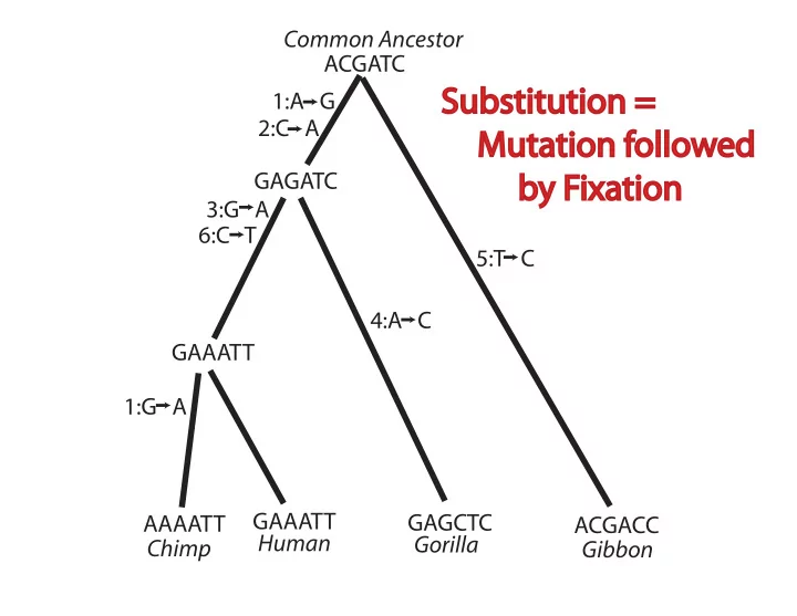
ACGATC GAGATC GAAATT AAAATT GAAATT GAGCTC ACGACC 5:T C 1:A G 2:C A 3:G A 6:C T 1:G A 4:A C Common Ancestor Chimp Human Gorilla Gibbon

Substitution = Mutation followed by Fixation

AAAATT GAAATT GAGCTC ACGACC Chimp Human Gorilla Gibbon

AAAATT GAAATT GAGCTC ACGACC Chimp Human Gorilla Gibbon AAAATT GAAATT GAGCTC ACGACC Chimp Human Gorilla Gibbon

Likelihood (Prob. of data given model & parameter values) = Likelihood for Site 1 X

AAAATT GAAATT GAGCTC ACGACC Chimp Human Gorilla Gibbon

Likelihood for Site 2 X

AAAATT GAAATT GAGCTC ACGACC Chimp Human Gorilla Gibbon

Likelihood for Site 6 ... X ... X ... X

G

AAAATT GAAATT GAGCTC ACGACC Chimp Human Gorilla Gibbon

G A

Probabilistic models of nucleotide change (independently and identically evolving sites) Let qij be the instantaneous rate of change at a site from nucleotide type i to j Q is matrix of instantaneous rates (Q will have 4 rows and 4 columns because i and j can each by any of 4 nucleotide types) For nucleotide starting as type i at time 0, probability nucleotide is type j at time t is denoted pij(t). pij(t) is referred to as a transition probability.

Consider a very very small amount of evolutionary time ∆t. When i = j, pij(∆t) . = qij∆t pii(∆t) . = 1 −

• j,j=i qij∆t

pii(∆t) . = 1 + qii∆t where qii = −

• j,j=i qij

(in preceding equations, . = can be replaced by = when the limit as ∆t approaches 0 is taken)

Jukes-Cantor model is simplest model of nucleotide substitution. It assumes sequence positions evolve independently and it assumes that all possible changes at a position are equally likely. Let πj be probability a residue is type j. πj is called the equilibrium probability of type j. pij(∞) = πj For Jukes-Cantor model, πj = 1/4 for all 4 nucleotide types j.

based on Figure 11 from Swofford et al. Chapter in Molecular Systematics (Sinauer, 2nd ed. 1996)

General Time Reversible Model Tamura-Nei SYM HKY85 K3ST Felsenstein 84 Felsenstein 81 Kimura 2 Param. Jukes-Cantor

Equal Base Frequencies Single Substitution Type 2 subst. types (transitions vs. transversions) Single Substitution Type 3 subst. types (transitions, 2 transversion classes ) Equal Base Frequencies 3 subst. types (transitions, 2 transversion classes) 2 subst. types (transitions vs. transversions)

Rate Matrix for Jukes-Cantor Model F R To O M A C G T A −3µ µ µ µ C µ −3µ µ µ G µ µ −3µ µ T µ µ µ −3µ Note 1: Diagonal matrix elements multiplied by −1 are rate away from nucleotide type of that row. Note 2: In later slide on Jukes-Cantor model, we write s/3 rather than µ.

Rate Matrix for Kimura 2-Parameter Model F R To O M A C G T A −α − 2β β α β C β −α − 2β β α G α β −α − 2β β T β α β −α − 2β Changes involving only purines (i.e., A and G) or only pyrimidines (i.e., C and T) are transitions. Changes in- volving one purine and one pyrimidine are transversions.

Rate Matrix for Felsenstein 1981 Model F R To O M A C G T A −µ(πC + πG + πT) µπC µπG µπT C µπA −µ(πA + πG + πT) µπG µπT G µπA µπC −µ(πA + πC + πT) µπT T µπA µπC µπG −µ(πA + πC + πG)

Rate Matrix for Hasegawa-Kishino-Yano (a.k.a. HKY or HKY85) Model

F R To O M A C G T A −µ(πC + κπG + πT) µπC µκπG µπT C µπA −µ(πA + πG + κπT) µπG µκπT G µκπA µπC −µ(κπA + πC + πT) µπT T µπA µκπC µπG −µ(πA + κπC + πG)

Rate Matrix for General Time Reversible Model

F R To O M A C G T A −µ(aπC + bπG + cπT) µaπC µbπG µcπT C µaπA −µ(aπA + dπG + eπT) µdπG µeπT G µbπA µdπC −µ(bπA + dπC + fπT) µfπT T µcπA µeπC µfπG −µ(cπA + eπC + fπG)

Time Reversibility is a common property of models

• f sequence evolution.

Time reversibility means that πipij(t) = πjpji(t) for all i, j, and t. πiqij = πjqji for all i and j. For phylogeny reconstruction, time reversibility means that we cannot (on the basis of sequence data alone) hope to distinguish which of two sequence is ancestral and which is the descendant.

The practical implication of time reversibility for phylogeny reconstruction is that maximum likelihood cannot infer the position of the root of the tree unless additional information information exists (e.g., which taxa are the outgroups) or additional assumptions are made (e.g., a molecular clock).

Q will represent matrix of instantaneous rates of change. For general time reversible model, entries of Q are:

To From A C G T A −(aπC + bπG + cπT ) aπc bπG cπT C aπA −(aπA + dπG + eπT ) dπG eπT G bπA dπC −(bπA + dπC + fπT ) fπT T cπA eπC fπG −(cπA + eπC + fπG)

In above matrix: a, b, c, d, e, and f cannot be

• negative. With any rate matrix (including above), the

transition probabilities P(t) can be determined from the rate matrix Q and the amount of evolution t via P(t) = eQt = I + (Qt) 1! + (Qt)2 2! + (Qt)3 3! + . . . , where I is the identity matrix.

Computing pij(t) for the Jukes-Cantor model The Jukes–Cantor model assumes that this is how nucleotide substitution occurs:

• 0. πA = πG = πC = πT = 1

4.

• 1. For each site in the sequence, an “event” will occur

with probability 4

3s per unit evolutionary time.

• 2. If no event occurs, the residue at the site does not

change.

• 3. If an event occurs, the probability that a residue is

type i after the event is πi.

What is the probability that no event occurs in t units

• f evolutionary time?

(1 − 4 3s) × (1 − 4 3s) × (1 − 4 3s) . . . (1 − 4 3s) = (1 − 4 3s)t. When 4

3s is close to 0,

1 − 4 3s . = e−4

3s.

Pr (no event) = (1 − 4 3s)t . = e−4

3st.

When s is redefined as an instantaneous rate per unit evolutionary time, the approximation becomes an equality: Pr (no event) = e−4

3st.

Pr (at least one event) = 1 − Pr (no event) = 1 − e−4

3st.

If there have been no “events”, then the residue cannot possibly have changed after an amount of evolution t. If there has been at least one event, then the residue is type j with probability πj. pii(t) = Pr (no events) + Pr (at least one event)πj = e−4

3st + (1 − e−4 3st)πj.

For i = j, pij(t) = Pr (at least one event)πj = (1 − e−4

3st)πj.

Notice that 4

3s and t appear only as a product. 4 3s and t

cannot be separately estimated. Only their product can be estimated. Note: A generalization of the Jukes–Cantor model, the “Felsenstein 1981” model does not require πA = πG = πC = πT = 1

4.

• Expected number of changes per site (branch length)

1 2 3 4 0.0 0.05 0.10 0.15 0.20 0.25

• Prob. of G at end of branch given A at beginning

Jukes-Cantor Transition Probabilities

• 1

2 3 4 0.4 0.6 0.8 1.0

Jukes-Cantor Transition Probabilities

• Prob. of A at end of branch given A at beginning

Expected number of changes per site (branch length)