
SLIDE 1
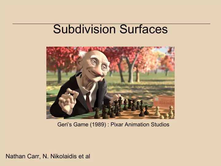
Subdivision Surfaces
Nathan Carr, N. Nikolaidis et al
Geri’s Game (1989) : Pixar Animation Studios
Subdivision Surfaces Geris Game (1989) : Pixar Animation Studios - - PowerPoint PPT Presentation
Subdivision Surfaces Geris Game (1989) : Pixar Animation Studios Nathan Carr, N. Nikolaidis et al Smooth versus General Polygon meshes are very general, but hard to model with In a production context (film, game), creating a dense,
Nathan Carr, N. Nikolaidis et al
Geri’s Game (1989) : Pixar Animation Studios
Process.
Refinement 1 Refinement 2 Refinement ∞ Note: Limit Curve/Surface not known!
Refinement
– Limit Surfaces/Curves will pass through original set of data points. – Each iteration generates only new vertices, does not move old
– Curve/Surface interpolates vertices from the previous step
– Limit Surface will not necessarily pass through the original set of data points.
– Create fair surfaces (smooth bends) – Converge faster – Shape is lowpass filtered, often shrinks!
– Less fairness, might create unnatural undulations – Creates mesh that usually is more “faithful” to the control mesh
2 1 3 2 1 2
3 2 5 3 2 4
1 1 1
1 1 2 1 2
+ + +
i i i i i i
Apply Iterated Function System Limit Curve
P0 P1 P2 P3 Q0 Q1 Q2 Q3 Q4 Q5
– Each edge must be split exactly once – Need to know endpoints of edge to create new vertex
– Require knowledge of which new edges to use – Require knowledge of new vertex locations
– Number of edges emanating from the vertex
8 3
8 1 8 3
8 1
2
1 nβ − β β β β β β
1 2 1 2 1 8 3 4 1 8
vertices: uniform in that respect)
sharp subdivision rules.
normal rules.
at a vertex
During Subdivision,
subdivision rules, according to the type of vertices.
– Smask is very sparse – Never Implement this way! – Allows for analysis
2 1 1 11 10 01 00
n nj mask
Smask Weights Old Control Points New Points
– In many cases subdivision surfaces converge to spline surfaces with C2 continuity everywhere.** – Too lengthy to cover here, but there is lots of literature.
Loop Subdivision Valence 6 Catmull-Clark Subdivision Valence 4
How should extraordinary vertices be handled?
“smooth”.
conforms to the original mesh (Moller book: w=0, d vertices do not participate)
⎭ ⎬ ⎫ ⎩ ⎨ ⎧ ⎥ ⎦ ⎤ ⎢ ⎣ ⎡ ⎟ ⎠ ⎞ ⎜ ⎝ ⎛ + ⎟ ⎠ ⎞ ⎜ ⎝ ⎛ + ≥ ⎭ ⎬ ⎫ ⎩ ⎨ ⎧ − = ⎭ ⎬ ⎫ ⎩ ⎨ ⎧ − − = N j N j N e v N e e e e v N e e e v N
j
π π 4 cos 2 1 2 cos 4 1 1 : , 4 3 : : 5 : , 8 1 : , : , 8 3 : , 4 3 : : 4 12 1 : , 12 1 : , 12 5 : , 4 3 : : 3 : Weights
3 2 1 2 1
Extraordinary Vertex New Edge vertex 1 ring neighborhood
formulas on the right (N=valence)
happen only in the first iteration) compute temporary vertices using formulas above, average to get new vertex.
1
m i i
=
Face Point Vertex Point
2 2 1 1
n n i i i i
= =
1 2 1 2
Edge Point
surface at every point except at these “extraordinary points”, and therefore at all but extraordinary points.
extraordinary points but note that trials indicate this much.
) 2 (
C
Pros:
Cons:
Geri’s Game (Pixar studios) Splines in Toy Story 1
need to be subdivided.
adaptively subdivide mesh where needed.
– Curvature – Screen size ( make triangles < size of pixel ) – View dependence
– Careful! Must ensure that “cracks” aren’t made crack subdivide View-dependent refinement of progressive meshes Hugues Hoppe. (SIGGRAPH ’87)
Computer Aided Design, Vol. 10, No. 6, pp 356-360, November 1978.
Section 13.4, Chapter 20.
Arbitrary Topology. Computer Graphics Proceedings (SIGGRAPH 96) (1996), 189–192.
Interpolation with Tension Control. ACM Trans. Gr. 9, 2 (April 1990), 160–169.
Department of Mathematics, 1987.