Student Responsibilities Reading : Textbook, Section 8.1, 8.3, 8.5 - - PDF document

Mat3770 — Relations

Spring 2014

Student Responsibilities

◮ Reading: Textbook, Section 8.1, 8.3, 8.5 ◮ Assignments:

Sec 8.1 1a-d, 3a-d, 5ab, 16, 28, 31, 48bd Sec 8.3 1ab, 3ab, 5, 14a-c, 18(ab), 23, 26, 36 Sec 8.5 2ad, 5, 15, 22, 35, 43a-c, 61

◮ Attendance: Spritefully Encouraged

Overview

◮ Sec 8.1 Relations and Their Properties ◮ Sec 8.3 Representing Relations ◮ Sec 8.5 Equivalence Relations

Section 8.1 — Relations and Their Properties

Binary Relations

◮ Definition: A binary relation R from a set A to a set B is a

subset R ⊆ A × B.

◮ Note: there are no constraints on relations as there are on

functions.

◮ We have a common graphical representation of relations, a

directed graph.

Directed Graphs

◮ Definition: A Directed Graph (Digraph) D from A to B is:

• 1. a collection of vertices V ⊆ A ∪ B, and
• 2. a collection of edges E ⊆ A × B

◮ If there is an ordered pair e =< x, y > in R, then there is an arc

• r edge from x to y in D. (Note: E = R)

◮ The elements x and y are called the initial and terminal vertices

• f the edge e.

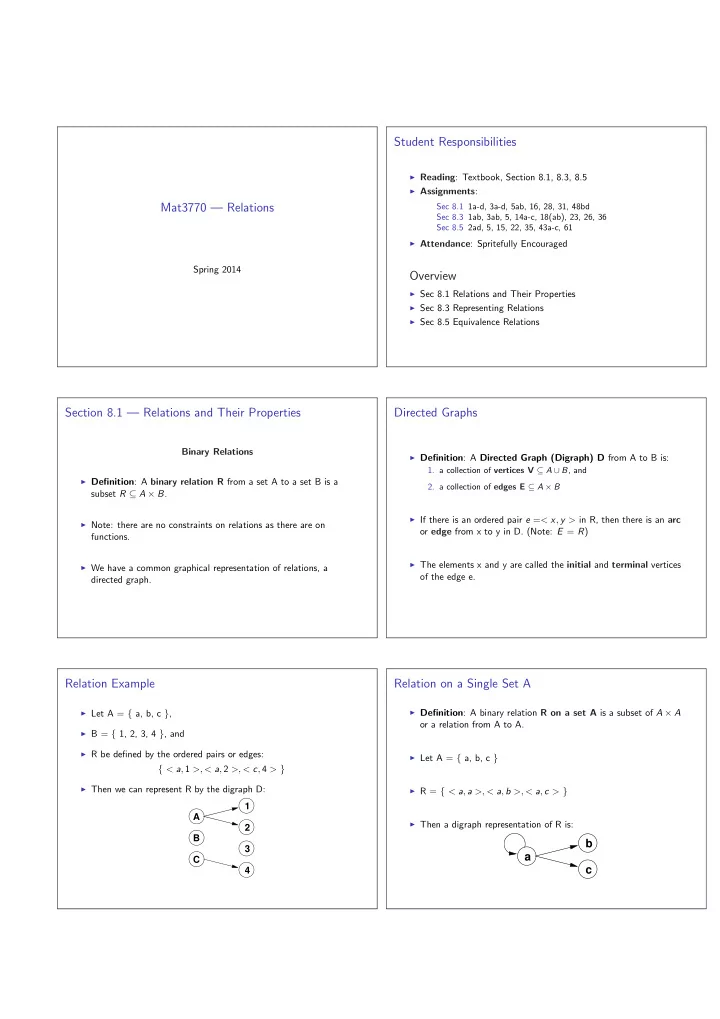
Relation Example

◮ Let A = { a, b, c }, ◮ B = { 1, 2, 3, 4 }, and ◮ R be defined by the ordered pairs or edges:

{ < a, 1 >, < a, 2 >, < c, 4 > }

◮ Then we can represent R by the digraph D:

A B C 1 2 3 4

Relation on a Single Set A

◮ Definition: A binary relation R on a set A is a subset of A × A

• r a relation from A to A.

◮ Let A = { a, b, c } ◮ R = { < a, a >, < a, b >, < a, c > } ◮ Then a digraph representation of R is:

a b c

Notes

◮ An arc of the form < x, x > on a digraph is called a loop. ◮ Question: How many binary relations are there on a set A?

Another way to think of it: How many subsets are there of A × A?

Special Properties of Binary Relations

Given

• 1. A universe U
• 2. A binary relation R on a subset A of U

◮ Definition: R is reflexive IFF

∀ x [x ∈ A → < x, x >∈ R]

◮ Notes:

◮ If A = ∅, then the implication is vacuously true ◮ The void relation on an empty set is reflexive ◮ If A is not void, then all vertices in the reflexive relation must have

loops

Symmetric and Antisymmetric Properties

◮ Definition: R is symmetric IFF

∀x∀y[< x, y >∈ R → < y, x >∈ R] Note: if there is an arc < x, y >, there must be an arc < y, x >

◮ Definition: R is antisymmetric IFF

∀x∀y[(< x, y >∈ R) ∧ (< y, x >∈ R) → x = y] Note: If there is an arc from x to y, there cannot be one from y to x if x= y. To prove a relation is antisymmetric, show logically that if < x, y > is in R and x = y, then < y, x > is not in R.

The Transitive Property

◮ Definition: R is transitive IFF

∀x∀y∀z[(< x, y >∈ R) ∧ (< y, z >∈ R) → < x, z >∈ R] Note: If there is an arc from x to y and one from y to z, then there must be one from x to z. This is the most difficult property to check. We will develop algorithms to check this later.

A B C D

R reflexive symmetric antisymmetric transitive A √ √ √ B C √ D √ √

Combining Relations — Set Operations

◮ A very large set of potential questions! For example, let R1 and

R2 be binary relations on a set A. Then we have questions of the form: If R1 has Property 1 and R2 has Property 2, does R1 ⋆ R2 have Property 3?

◮ For example, If R1 is symmetric and R2 is antisymmetric, does it

follow that R1 ∪ R2 is transitive? If so, we need to prove it;

• therwise, we can find a counterexample.

Another Example

◮ Let R1 and R2 be transitive on A. Does it follow that R1 ∪ R2 is

transitive?

◮ Consider:

◮ A = { 1, 2 } ◮ R1 = { < 1, 2 > } ◮ R2 = { < 2, 1 > }

◮ Then R1 ∪ R2 = { < 1, 2 >, < 2, 1 > }. which is not transitive.

(Why not?)

Composition of Relations

◮ Definition: Suppose

◮ R1 is a relation from A to B ◮ R2 is a relation from B to C

Then the composition of R2 with R1, denoted R2 ◦ R1, is the relation from A to C: If < x, y > is a member of R1 and < y, z > is a member of R2 , then < x, z > is a member of R2 ◦ R1

◮ For < x, y > to be in the composite relation R2 ◦ R1, there

must exist a y in B

◮ We read compositions right to left as in functions, applying R1

first, then R2 in this example.

Example of a Composite Relation

B C 1 2 3 4 R1 R2 A

R2 ◦ R1 = { < B, 2 >, < B, 4 > }

A Relation Composed with Itself

◮ Definition: Let R be a binary relation on A. Then the powers

Rn, n = 1, 2, 3, . . . are defined recursively by:

◮ Basis: R1 = R ◮ Induction: Rn+1 = Rn ◦ R

◮ Note: An ordered pair < x, y > is in Rn IFF there is a path of

length n from x to y following the arcs (in the direction of the arrows) in R.

Composites on R R R R R

3 2= R 1 R 4 = R R 3

= R

1

= R R

2

A Very Important Theorem

R is transitive IFF Rn ⊆ R for n > 0.

Proof ( ⇒ ): R transitive → Rn ⊆ R Use a direct proof with proof by induction

◮ Assume R is transitive & show Rn ⊆ R by induction

Basis: Obviously true for n = 1 Induction:

◮ IH: Assume Rk ⊆ R for some arbitrary k > 0 ◮ IS: Show Rk+1 ⊆ R

Rk+1 = Rk ◦ R, so if < x, y > is in Rk+1, then there is a z such that < x, z > is in Rk and < z, y > is in R. But, since Rk ⊆ R, < x, z > is in R R is transitive, so < x, y > is in R Since < x, y > was an arbitrary edge, the result follows

Proof ( ⇐ )

To complete the proof, we need to show: Rn ⊆ R → R is transitive Use the fact that R2 ⊆ R and the definition of transitivity. Proof left as an exercise. . . Thus, (given a finished proof of the above) we have shown: R is transitive IFF Rn ⊆ R for n > 0

Section 8.3 — Representing Relations

Connection Matrices

◮ Let R be a relation from A = { a1, a2, . . . , am } to

B = { b1, b2, . . . , bn }

◮ Definition: An m × n connection matrix, M, for R is defined

by: mi,j = 1 if < ai, bj > ∈ R

• therwise

Example

◮ Assume the rows are labeled with the elements of A and the

columns are labeled with the elements of B.

Let A = { a, b, c }, B = { e, f, g, h }, and R = { < a, e >, < c, g > }

◮ Then the connection matrix M for R is:

  1 1  

◮ Note: The order of the elements of A and B is important!

• Theorem. let R be a binary relation on a set A and let M be its

connection matrix. Then:

◮ R is reflexive IFF Mi,i = 1 for all 1 ≤ i ≤ |A| ◮ R is symmetric IFF M is a symmetric Matrix: M = MT ◮ R is antisymmetric if Mij = 0 or Mji = 0 for all i = j

Combining Connection Matrices — Join

◮ Definition: The join of two matrices, M1 and M2, denoted

M1 ∨ M2, is the component–wise Boolean ”or” of the two matrices.

◮ Fact: If M1 is the connection matrix for R1, and M2 is the

connection matrix for R2, then the join of M1 and M2, M1 ∨ M2, is the connection matrix for R1 ∪ R2

Combining Connection Matrices — Meet

◮ Definition:The meet of two matrices, M1 and M2, denoted

M1 ∧ M2, is the component–wise Boolean ”and” of the two matrices.

◮ Fact: If M1 is the connection matrix for R1, and M2 is the

connection matrix for R2, then the meet of M1 and M2, M1 ∧ M2, is the connection matrix for R1 ∩ R2

Finding Connection Matrix Combinations

Given the connection matrix for two relations, how does one find the connection matrix for:

◮ The complement: (A × A) − R ◮ The relative complement: R1 − R2 and R2 − R1 ◮ The symmetric difference: R1 ⊕ R2 = (R1 − R2) ∪ (R2 − R1)

The Composition

◮ Definition: Let M1 be the connection matrix for R1, and M2 be

the connection matrix for R2. Then the Boolean product of these two matrices, denoted M1 ⊗ M2, is the connection matrix for the composition of R2 with R1, R2 ◦ R1 (M1 ⊗ M2)ij = ∨n

k=1[(M1)ik ∧ (M2)kj)] ◮ Why? In order for there to be an arc < x, z > in the composition,

then there must be an arc < x, y > in R1 and an arc < y, z > in R2 for some y.

Notes on Composition

◮ The Boolean product checks all possible y’s. If at least one such

path exists, that is sufficient.

◮ The matrices M1 and M2 must be conformable: the number of

columns of M1 must equal the number of rows of M2.

◮ If M1 is m × n and M2 is n × p, then M1 ⊗ M2 is m × p

Composition Example — R2 ◦ R1

R R

1 2

A B C

1 2 3 1 2 3 4 1 2 M2= 0 0 0 1 1 0 0 1

1

M 0 0 0 1 0 1 0 0 0 1 0 0 =

1

M M2 = 0 1 0 1 0 1

(M1 ⊗ M2)12 = [(M1)11 ∧ (M2)12] ∨ [(M1)12 ∧ (M2)22] ∨ [(M1)13 ∧ (M2)32] ∨ [(M1)14 ∧ (M2)42] ∨ = [0 ∧ 0] ∨ [1 ∧ 1] ∨ [0 ∧ 0] ∨ [0 ∧ 1] = 1

◮ There is an arc in R1 from node 1 in A to node 2 in B ◮ There is an arc in R2 from node 2 in B to node 2 in C ◮ Hence, there is an arc in R2 ◦ R1 from node 1 in A to node 2 in C. ◮ A useful result: MRn = (MR)n

Digraphs

Given the digraphs for R1 and R2, describe how to find the digraphs for:

◮ Union: R2 ∪ R1 ◮ Intersection: R2 ∩ R1 ◮ Relative Complement: R2 − R1 ◮ Boolean Product: R2 ⊗ R1 ◮ Complement: A × A − R1 ◮ Symmetric Difference: R1 ⊕ R2

Section 8.5 — Equivalence Relations

Wherein we define new types of important relations by grouping properties of relations together. Definition: A relation R on a set A is an equivalence relation IFF R is:

◮ reflexive ◮ symmetric, and ◮ transitive

Equivalence Relations in Digraphs

Equivalence relations are easily recognized in digraphs

◮ The set of all elements related to a particular element forms a

subgraph in which all self–loops and arcs are present between the included vertices.

◮ I.e., the digraph (or subdigraph) representing the subset will be a

complete digraph (or subdigraph).

◮ The number of such subsets is called the rank of the equivalence

relation.

All Equivalence Relations on a Set with 3 Elements

rank = 1 rank = 2 rank = 3 rank = 2 rank = 2

Equivalence Classes

◮ Each complete subset is called an equivalence class. ◮ A bracket around an element means the equivalence class in

which the element lies. [x] = {y| < x, y >∈ R}

◮ The element in the bracket is called a representative of the

equivalence class — we could have chosen any element in that class.

◮ Three ways to say ”in the same equivalence class”:

aRb [a] = [b] [a] ∩ [b] = ∅

Example — Equivalence Classes

a b c

[a] = {a, c}, [c] = {a, c}, [b] = {b} rank = 2

Partitions

◮ Definition: Let S1, S2, . . . , Sn be a collection of subsets of A.

Then the collection forms a partition of A if the subsets are non–empty, disjoint, and exhaust A. Si = ∅ Si ∩ Sj = ∅ if i = j Si = A

S1 S3 S2 S4 S5

A

• Theorem. The equivalence classes of an equivalence relation R

partition the set A into disjoint nonempty subsets whose union is the entire set. The partition is denoted A/R and is called:

◮ the quotient set or ◮ the partition of A induced by R, or ◮ A modulo R

Examples

• 1. The set of integers such that aRb IFF a = b or a = −b
• 2. The natural numbers mod any integer:

For example, N mod 3 divides the natural numbers into 3 equivalence classes: [0]3, [1]3, [2]3 3.

a b c

[a] = {a}, [b] = {b, c}, [c] = {b, c} rank = 2

• Theorem. Let R be an equivalence relation on A. Then either

[a] = [b]

• r

[a] ∩ [b] = ∅ Why?

Review — R ⊆ A × A

◮ reflexive: (a, a) ∈ R ∀ a ∈ A ◮ symmetric: (b, a) ∈ R ↔ (a, b) ∈ R for a, b ∈ A ◮ antisymmetric:

(b, a) ∈ R and (a, b) ∈ R, then a = b for a, b ∈ A

◮ transitive:

(a, b) ∈ R and (b, c) ∈ R, then (a, c) ∈ R for a, b, c ∈ A

Transitive Closure

◮ A path in a digraph is a sequence of connected edges. ◮ A path has length n, where n is the number of edges in the path. ◮ A circuit or cycle is a path that begins and ends at the same

vertex.

◮ The connectivity relation R⋆ is the set of all pairs <a, b> such

that there is a path between a and b in the relation R. This is also called the transitive closure of R.

• Theorem. If R1 and R2 are equivalence relations on A, then

R1 ∩ R2 is an equivalence relation on A. Proof outline: It would suffice to show that the intersection of:

◮ reflexive relations is reflexive ◮ symmetric relations is symmetric, and ◮ transitive relations is transitive

Reflexive, Symmetric, Transitive Closure

• Definition. Let R be a relation on A. Then the reflexive,

symmetric, transitive closure of R, denoted tsr(R), is an equivalence relation induced by R on A. Example: tsr(R), rank = 2 a b c d R a b c d A/R = { {a}, {b, c, d} } A = [a] [b] = {a} {b, c, d}

• Theorem. tsr(R) is an equivalence relation.
• Proof. We must be careful and show that tsr(R) is still symmetric

and reflexive.

◮ Since we only add arcs (rather than delete arcs) when computing

closures, it must be that tsr(R) is reflexive since all loops < x, x > on the digraph must be present when constructing r(R).

◮ If there is an arc < x, y >, then the symmetric closure of r(R)

ensures there is an arc < y, x >.

◮ We may now argue that if we construct the transitive closure of

sr(R) and we add an edge < x, z > because there is a path from x to z, then there must also exist a path from z to x, and hence we also must add an edge < z, x >. Hence the transitive closure

• f sr(R) is symmetric.