Structural analysis for fault diagnosis faults f ( t ) observation y - - PowerPoint PPT Presentation

Structural analysis for fault diagnosis

• f equation based models

Erik Frisk <erik.frisk@liu.se> Department of Electrical Engineering Linköping University, Sweden

Jubilee Symposium — Future Direc4ons of System Modeling and Simula4on


• Sept. 30, Lund, Sweden

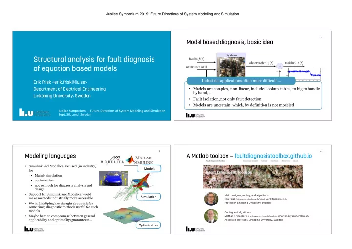
Model based diagnosis, basic idea

2

System Model ˙ x = g(x, u) y = h(x, u) + faults f(t) actuators u(t)

• bservation y(t)

prediction ˆ y(t) residual r(t) −

5 10 15 20 25 30 35 40 45 −1 −0.5 0.5

Industrial applications often more difficult …

• Models are complex, non-linear, includes lookup-tables, to big to handle

by hand, …

• Fault isolation, not only fault detection
• Models are uncertain, which, by definition is not modeled

Modeling languages

• Simulink and Modelica are used (in industry)

for

• Mainly simulation
• optimization
• not so much for diagnosis analysis and

design

• Support for Simulink and Modelica would

make methods industrially more accessible

• We in Linköping has thought about this for

some time; diagnostic methods useful for such models

• Maybe have to compromise between general

applicability and optimality/guarantees/…

3

Models Simulation Optimization

A Matlab toolbox — faultdiagnosistoolbox.github.io

4

Main designer, coding, and algorithms Erik Frisk (http://users.isy.liu.se/fs/frisk/) <erik.frisk@liu.se> Professor, Linköping University, Sweden Coding and algorithms Mattias Krysander (http://users.isy.liu.se/fs/matkr/) <mattias.krysander@liu.se> Associate professor, Linköping University, Sweden

Jubilee Symposium 2019: Future Directions of System Modeling and Simulation

Basic approach to diagnosis system design

5

Model Sub-model
 With
 Redundancy Residual
 Generator

DAEs and equation based models for diagnosis

• Non-causal models — inherent in the diagnosis problem
• A signal is known or unknown; it does not matter if it is an input or
• utput signal to the system
• — unknown, known, and fault signals

• Submodels — inherently differential-algebraic


x, z, f F(· x, x, z, f ) = 0 · x1 = f1(x1, x2, z, f ) · x2 = f2(x1, x2, z, f ) y1 = h1(x1, x2, z, f ) y2 = h2(x1, x2, z, f )

6

· x1 = f1(x1, x2, z, f ) y1 = h1(x1, x2, z, f )

Differential index and diagnosis filter design

• Standard definition on differential index is for just-determined models but

can be directly extended to over-determined models, i.e., models with redundancy,


• If sub-model is low-index, standard observer design techniques can be

utilized for a fault detector in the form


• Thus low-index sub-models are of particular interest for detector synthesis

· x1 = f1(x1, x2, z, f ) y1 = h1(x1, x2, z, f ) ·̂ x1 = g1( ̂ x1, ̂ x2, z) + Kgr( ̂ x1, ̂ x2, z) 0 = ga( ̂ x1, ̂ x2, z) r = gr( ̂ x1, ̂ x2, z)

7

Structural models

8

Structural model A structural model only models that variables are related! Example relating variables: V , i, ω e1 : V = iR(1 + fR) + L di dt + Kai ω

Unknown variables i θ ω α T Tm Tl fR fi fω fT V yi yω yT e1 X X X X

Coarse model description, no parameters or analytical expressions Can be obtained early in design process with little engineering effort Large-scale model analysis possible using graph theoretical tools Very useful!

Jubilee Symposium 2019: Future Directions of System Modeling and Simulation

Structural representation of engine model

9 e1 e2 e3 e4 e5 e6 e7 e8 e9 e10 e11 e12 e13 e14 e15 e16 e17 e18 e19 e20 e21 e22 e23 e24 e25 e26 e27 e28 e29 e30 e31 e32 e33 e34 e35 e36 e37 e38 e39 e40 e41 e42 e43 e44 e45 e46 e47 e48 e49 e50 e51 e52 e53 e54 e55 e56 e57 e58 e59 e60 e61 e62 e63 e64 e65 e66 e67 e68 e69 e70 e71 e72 e73 e74 e75 e76 e77 e78 e79 e80 e81 e82 e83 e84 e85 e86 e87 e88 e89 e90 e91 e92 e93 e94 Engine model

D I D I D I D I D I D I D I D I D I D I D I D I D I D I

W_af p_t W_es p_ic T_ic W_ic W_th Aeff_th W_wg Aeff_wg T_af p_af W_c T_cout T_c p_c T_imcr p_im T_im W_e T_ti T_em p_em dh_is W_twg T_turb T_t alpha_th

• mega_e

W_ig W_fr Tq_c eta_c

• mega_tc

PSI_c PI_c W_t Tq_t eta_t PI_t u_wg wg_pos DELTA_theta T_e T_amb p_amb PSI_th PI_wg PSIli_wg m_af m_c m_ic T_fwd_flow_ic m_im m_em m_t PI_cnolim U_c PHI_model W_ccorr Tq_e_cs Tq_e_cb Tq_e_f Tq_e_p eta_ign W_i_p FMEP S_p BMEP C_eta_vol T_in eta_vol W_ac W_fc T_tout Tflow_wg dmdt_af dTdt_af dmdt_c dTdt_c dmdt_ic dTdt_ic dmdt_im dTdt_im dmdt_em dTdt_em dmdt_t dTdt_t domegadt_tc dwgdt_pos fp_af fw_af fw_th fw_c fc_vol fw_t fx_th fyw_af fyp_im fyp_ic fyT_ic y_p_ic y_p_im y_T_ic y_W_af y_omega_e y_alpha_th y_u_wg y_wfc y_T_amb y_p_amb

• Incidence matrix of variable

dependency graph

• Edges represents connections
• I/D-edges correspond to

differentiation and integration

Fundamental algorithmic tool: Dulmage-Mendelsohn decomposition

• Basic tool in many structural

analysis algorithms

• Smart reordering or

rows(equations) and columns (variables)

• Partitions the model into three

parts

• Under determined
• Exactly determined
• Over determined
• The overdetermined part with

redundancy is the one interesting for diagnosis

10 b0 b1 b2 ... bn−1 bn b∞ X0 X1 X2 · · · Xn−1 Xn X∞ M − M 0 M +

Outline of the talk

• 1. Diagnosability and sensor placement analysis
• 2. Testable (sub-)models and detector synthesis
• 3. A Modelica perspective
• 4. An automotive use-case

11

Presentation will be more what than how

Diagnosability analysis and sensor selection

Jubilee Symposium 2019: Future Directions of System Modeling and Simulation

Diagnosability analysis - Problem formulation

• Given a dynamic model
• Q1: Which faults are

structurally detectable?

• Q2: What are the structural

isolability properties of the model?

13 e1 e2 e3 e4 e5 e6 e7 e8 e9 e10 e11 e12 e13 e14 e15 e16 e17 e18 e19 e20 e21 e22 e23 e24 e25 e26 e27 e28 e29 e30 e31 e32 e33 e34 e35 e36 e37 e38 e39 e40 e41 e42 e43 e44 e45 e46 e47 e48 e49 e50 e51 e52 e53 e54 e55 e56 e57 e58 e59 e60 e61 e62 e63 e64 e65 e66 e67 e68 e69 e70 e71 e72 e73 e74 e75 e76 e77 e78 e79 e80 e81 e82 e83 e84 e85 e86 e87 e88 e89 e90 e91 e92 e93 e94 Engine model

D I D I D I D I D I D I D I D I D I D I D I D I D I D I

W_af p_t W_es p_ic T_ic W_ic W_th Aeff_th W_wg Aeff_wg T_af p_af W_c T_cout T_c p_c T_imcr p_im T_im W_e T_ti T_em p_em dh_is W_twg T_turb T_t alpha_th

• mega_e

W_ig W_fr Tq_c eta_c

• mega_tc

PSI_c PI_c W_t Tq_t eta_t PI_t u_wg wg_pos DELTA_theta T_e T_amb p_amb PSI_th PI_wg PSIli_wg m_af m_c m_ic T_fwd_flow_ic m_im m_em m_t PI_cnolim U_c PHI_model W_ccorr Tq_e_cs Tq_e_cb Tq_e_f Tq_e_p eta_ign W_i_p FMEP S_p BMEP C_eta_vol T_in eta_vol W_ac W_fc T_tout Tflow_wg dmdt_af dTdt_af dmdt_c dTdt_c dmdt_ic dTdt_ic dmdt_im dTdt_im dmdt_em dTdt_em dmdt_t dTdt_t domegadt_tc dwgdt_pos fp_af fw_af fw_th fw_c fc_vol fw_t fx_th fyw_af fyp_im fyp_ic fyT_ic y_p_ic y_p_im y_T_ic y_W_af y_omega_e y_alpha_th y_u_wg y_wfc y_T_amb y_p_amb b0 b1 b2 ... bn−1 bn b∞ X0 X1 X2 · · · Xn−1 Xn X∞ M0 M1 M2 . . . Mn−1 Mn M∞ f1 f2

Structurally detectable and isolable faults

• Let

be the equation that is affected by fault

• A fault is (structurally) detectable iff

• Fault not detectable, is detectable
• A fault is isolable form a fault iff

• Take home: Structural diagnosability can be 


determined by a series of 
 Dulmage-Mendelsohn decompositions (fast)

efi fi fi efi ∈ M+ f1 f2 fi fj efi ∈ (M∖efj)+

14

Diagnosability of an engine model

15

fp_af fw_af fw_th fw_c fc_vol fw_t fx_th fyw_affyp_imfyp_ic fyT_ic fp_af fw_af fw_th fw_c fc_vol fw_t fx_th fyw_af fyp_im fyp_ic fyT_ic Isolability matrix for 'Engine model'

Injected fault Diagnoses

A more detailed structure decomposition

16 100 200 300 400 500 600 700 800 Variables 100 200 300 400 500 600 700 800 Equations Dulmage-Mendelsohn decomposition of model 'SECS'

D I D I D I D I D I D I D ID I D I D I D I D I D ID ID I D I D I D I D I D I D I D I D I

f1 f2 f3 f4 f5 f6 f7 f8 f9 f10 f11 f12 f13 f14 f15 f16 f17 f18 f19 f20 f21 f22 0 50 100 150 200 250 300 350 400 450 500 550 600 650 700 750 800 850 Variables 50 100 150 200 250 300 350 400 450 500 550 600 650 700 750 800 850 Equations Dulmage-Mendelsohn decomposition of model 'SECS'

D I D I D I D I D I D I D ID I D I D I D I D I D ID ID I D I D I D I D I D I D I D I D I D I D I D I D I D I D I D ID I D I D I D I D I D ID ID I D I D I D I D I D I D I D I D I

f1 f2 f3 f4 f5 f6 f7 f8 f9 f10 f11 f12 f13 f14 f15 f16 f17 f18 f19 f20 f21 f22

Jubilee Symposium 2019: Future Directions of System Modeling and Simulation

Isolability and a more detailed structure decomposition

17 f21f22 f1 f5 f7 f8 f2 f3 f4 f6 f9 f17f10f11f12f13f16f14f15f18f19f20 f21 f22 f1 f5 f7 f8 f2 f3 f4 f6 f9 f17 f10 f11 f12 f13 f16 f14 f15 f18 f19 f20 Interpreted faults Isolability matrix Injected fault 500 550 600 650 700 750 800 850 Variables 500 550 600 650 700 750 800 850 Equations Dulmage-Mendelsohn decomposition of model 'SECS'

D I D I D I D I D ID ID I D I D ID I D I D I D I D I D I D I D ID ID I D I D ID I D I D I

f1 f2 f3 f4 f5 f6 f7 f8 f9 f10 f11 f12 f13 f14 f15 f16 f17 f18 f19 f20 f21 f22

18

Minimal sensor sets and problem formulation

Given: A set P of possible sensor locations A detectability and isolability performance specification Minimal Sensor Set A multiset S, defined on P, is a minimal sensor set if the specification is fulfilled when the sensors in S are added, but not fulfilled when any proper subset is added. Problem Statement Find all minimal sensor sets with respect to a required isolability specification and possible sensor locations for any linear differential-algebraic model

x1 x2 x3 x4 x5 e5 e4 e3 e2 e1 f1 f2 f3 f4 b1 b2 b3 b4 b5

⇒

b1 b2 b3 b4 b5

x1 x2 x3 x4 x5 e5 e4 e3 e2 e1 f1 f2 f3 f4 e6 b1 b2 b3 b4 b5

⇒

b1 b2 b3 b4 b5

Basic principle for finding sensors

19

• 1. A Dulmage-Mendelsohn decomposition (again)
• 2. Define a partial order on equations that explicitly identifies variables to

measure

Example: An electrical circuit

A small electrical circuit with 5 components that may fail

z C R2

1

R1 L

2 4 5 3

20

Jubilee Symposium 2019: Future Directions of System Modeling and Simulation

21

Example: An electrical circuit

A small electrical circuit with 5 components that may fail

z C R2

1

R1 L

2 4 5 3

v1 = v5 v5 = v2 + v3 i1 = i2 + i5 i1 = i3 + i4 + i5 v1 = z v2 = R1i2 v4 = L d dt i4 i5 = C d dt v5 v3 = v4 v3 = R2i3 10 equations, 2 states, 5 faults, 1 known signal Possible measurements: currents and voltages

22

Examples of results of the analysis

C R2

1

R1 L

2 4 5 3

z Example run 1 Objective Achieve detectability Possible measurement voltages and currents 7 minimal solutions {i1} , {i2, i5}, {i3, i5}, {i4, i5}, {i5, v2}, {i5, v3}, {i5, v4}

23

Examples of results of the analysis

C R2

1

R1 L

2 4 5 3

z Example run 2 Objective Achieve full isolability Possible measurement voltages and currents 5 minimal solutions {i1, i3} , {i1, i4}, {i2, i3, i5}, {i2, i4, i5}, {i3, i4, i5}

24

Examples of results of the analysis

C R2

1

R1 L

2 4 5 3

z Example run 3 Objective Achieve full isolability, new sensors may fail Possible measurement voltages and currents 7 minimal solutions {i1, i1, i3} , {i1, i1, i4}, {i1, i3, i5}, {i1, i4, i5}, {i2, i3, i5, i5}, {i2, i4, i5, i5}, {i3, i4, i5, i5}

186 / 226

Jubilee Symposium 2019: Future Directions of System Modeling and Simulation

Testable sub-models and detector synthesis Model based diagnosis, basic ideas

26

System Model ˙ x = g(x, u) y = h(x, u) + faults f(t) actuators u(t)

• bservation y(t)

prediction ˆ y(t) residual r(t) −

Model

Sub-model
 with
 Redundancy Residual
 Generator

27

Basic principle - systematic utilization of redundancy

1 equation, 1 unknown, no redundancy x = g(u)

28

Basic principle - systematic utilization of redundancy

2 equations, 1 unknown, 1 residual generator x = g(u) r1 = y1 − g(u) y1 = x Jubilee Symposium 2019: Future Directions of System Modeling and Simulation

29

Basic principle - systematic utilization of redundancy

3 equations, 1 unknown, 3 residual generators x = g(u) r1 = y1 − g(u) y1 = x r2 = y2 − g(u) y2 = x r3 = y2 − y1

30

Basic principle - systematic utilization of redundancy

4 equations, 1 unknown, 6 (minimal) residual generators x = g(u) r1 = y1 − g(u) y1 = x r2 = y2 − g(u) y2 = x r3 = y2 − y1 y3 = x r4 = y3 − g(u) r5 = y3 − y1 r6 = y3 − y2

31

Basic principle - systematic utilization of redundancy

4 equations, 1 unknown, 6 (minimal) residual generators x = g(u) r1 = y1 − g(u) y1 = x r2 = y2 − g(u) y2 = x r3 = y2 − y1 y3 = x r4 = y3 − g(u) r5 = y3 − y1 r6 = y3 − y2 Number of possibilities grows exponentially (here n

2

• minimal

combinations) Not just y − ˆ y Is this illustration relevant for more general cases? Answer:
 Very much so, but careful analysis of DAE equations and their properties is essential

Basic approach to diagnosis system design

32

Model Sub-model
 With
 Redundancy Residual
 Generator How do you do this step?

Jubilee Symposium 2019: Future Directions of System Modeling and Simulation

Sketch — how to find all minimal models with redundancy

33

Model Sub-model

M+

Sub-model

M+

Minimal model with redundancy

• Do this systematically; efficient way to find all MSO sets — Minimal

Structurally Overdetermined set of equations

• A series of Dulmage-Mendelsohn operations — efficient
• Exponential in model redundancy — extensions for MSO exists to reduce

solution set

A Modelica perspective Is Modelica a good language for this kind of analysis

• Started two masters theses together with Saab, Linköping
• Demonstrate automatic transformation of Modelica models into a format

where existing fault diagnosis techniques are applicable.

• Describe how to make non-trivial diagnosis analysis for non-trivial

Modelica models.

35

Use-case: Environmental Cooling System for Gripen Aircraft

• Modelica model
• Uses standard libraries
• 1,000 - 10,000 equations

36

f2 f3 f5 f6 f7 f8 f1 f4 f9 f12 f13 f14 f15 f16 f17 f18 f20 f19 f21 f22

15 sensors (temp, pres, rot)

Jubilee Symposium 2019: Future Directions of System Modeling and Simulation

Modelica and structural analysis

• Flat Modelica model is well suited

for structural analysis

• Structural analysis requires non-

repeated expressions

• Connecting components give, by

construction, non-repeated expressions if the model is not simplified.

• State-space forms are typically not

suitable

37

100 200 300 400 500 600 700 800 900 100 200 300 400 500 600 700 800 Variables

D I D I D I D I D I D I D I D I D I D ID I D I D I D I D I D ID I D I D I D I D I D I D I

Structural model Equations

Toolchain

38

1 <SimpleEquation>

<LHS>

3

<ComponentReference> <Reference

5

instanceName=”y”/> </ComponentReference>

7

</LHS> <RHS>

9

<Binary Operator=”+”> <Left>

11

<ComponentReference> <Reference

13

instanceName=”x”/> </ComponentReference>

15

</Left> <Right>

17

<Literal Value=”1”/> </Right>

19

</Binary> </RHS>

21 </SimpleEquation>

Modelica XML representation XML to FDT- format parser Analysis in Matlab

y = x + 1 Modelica model with faults

39

f2 f3 f5 f6 f7 f8 f1 f4 f9 f12 f13 f14 f15 f16 f17 f18 f20 f19 f21 f22

f12 f13 f14 f15 f16 f17 f18 f20 f19

Straightforward to extend existing components with fault models

Transformation: .mo → XML → .m

40

f2 f3 f5 f6 f7 f8 f1 f4 f9 f12 f13 f14 f15 f16 f17 f18 f20 f19 f21 f22

Dymola

A few hundred lines of Python-code

Jubilee Symposium 2019: Future Directions of System Modeling and Simulation

Conditionals

• Very common with conditionals in more complex models
• Common in the ECS model here
• Related to hybrid/switched systems
• Here a simple, and pragmatic approach

41

if c(xc) > 0 then

2

x1 = g1(x2); else

4

x1 = g2(x2, x3); end if;

x1 = if(c(xc) > 0; g1(x2); g2(x2, x3)) = f(xc, x2, x3)

Model structure

• Gripen Environmental

Cooling System model

• 884 equations, 23

dynamic states

• 22 faults
• Degree of redundancy 15


42 100 200 300 400 500 600 700 800 900 100 200 300 400 500 600 700 800 Variables

D I D I D I D I D I D I D I D I D I D ID I D I D I D I D I D ID I D I D I D I D I D I D I

Structural model Equations

Isolability from structure

43 f21f22 f1 f5 f7 f8 f2 f3 f4 f6 f9 f17f10f11f12f13f16f14f15f18f19f20 f21 f22 f1 f5 f7 f8 f2 f3 f4 f6 f9 f17 f10 f11 f12 f13 f16 f14 f15 f18 f19 f20 Interpreted faults Isolability matrix Injected fault 500 550 600 650 700 750 800 850 Variables 500 550 600 650 700 750 800 850 Equations Dulmage-Mendelsohn decomposition of model 'SECS'

D I D I D I D I D ID ID I D I D ID I D I D I D I D I D I D I D ID ID I D I D ID I D I D I

f1 f2 f3 f4 f5 f6 f7 f8 f9 f10 f11 f12 f13 f14 f15 f16 f17 f18 f19 f20 f21 f22

Residual generator properties

44

10 20 30 40 50 60 70 80 90 100 110 120 130 50 100 150 200 250 300 4 states 3 states 1 states redundancy 1 redundancy 2 redundancy 2 redundancy 2 redundancy 2 PSO set Number of equations 0 states f1 f2 f3 f4 f5 f6 f7 f8 f9 f10 f11 f12 f13 f14 f15 f16 f17 f18 f19 f20 f21 f22 5 79 80 27 14 1 24 90 48 65 fault PSO set Fault signature matrix

• Test selection to achieve maximum single fault

isolability by a Greedy search:

• 1) Few states 2) Few equations
• 10 tests with maximum single fault isolability

Jubilee Symposium 2019: Future Directions of System Modeling and Simulation

Summary

• Straightforward to transfer Modelica models to analysis format (Matlab)
• Here a limited part of the Modelica language
• Toolchain via XML representation (unfortunately, not standardized)


• Possible to obtain non-trivial results
• Fault detectability, fault isolability, fault detector analysis
• Saab developers also appreciate:
• Gain additional insight in model structure
• Find model weaknesses using fault diagnosis techniques

45

Modelica XML representation XML to FDT- format parser Analysis in Matlab

An automotive use-case

Volvo development control system We can inject, physically and through the control system, many relevant faults

Jubilee Symposium 2019: Future Directions of System Modeling and Simulation

Test cell data

• Volvo production engine
• EPA HWFET cycle translated into load

cycle for engine (rpm/torque)

• (here) 5 data sets:
• 1. Fault free
• Sensor faults
• 2. Intake pressure
• 3. Air-flow sensor
• 4. Pressure after intercooler
• 5. Temperature after intercooler

49

2 4 6 8 10 12 14 t [min] 10 20 30 40 50 60 70 80 90 100 Velocity [km/h] EPA Highway Fuel Economy Test Cycle (HWFET)

Structural model of the engine

50 e1 e2 e3 e4 e5 e6 e7 e8 e9 e10 e11 e12 e13 e14 e15 e16 e17 e18 e19 e20 e21 e22 e23 e24 e25 e26 e27 e28 e29 e30 e31 e32 e33 e34 e35 e36 e37 e38 e39 e40 e41 e42 e43 e44 e45 e46 e47 e48 e49 e50 e51 e52 e53 e54 e55 e56 e57 e58 e59 e60 e61 e62 e63 e64 e65 e66 e67 e68 e69 e70 e71 e72 e73 e74 e75 e76 e77 e78 e79 e80 e81 e82 e83 e84 e85 e86 e87 e88 e89 e90 e91 e92 e93 e94 Engine model

D I D I D I D I D I D I D I D I D I D I D I D I D I D I

W_af p_t W_es p_ic T_ic W_ic W_th Aeff_th W_wg Aeff_wg T_af p_af W_c T_cout T_c p_c T_imcr p_im T_im W_e T_ti T_em p_em dh_is W_twg T_turb T_t alpha_th

• mega_e

W_ig W_fr Tq_c eta_c

• mega_tc

PSI_c PI_c W_t Tq_t eta_t PI_t u_wg wg_pos DELTA_theta T_e T_amb p_amb PSI_th PI_wg PSIli_wg m_af m_c m_ic T_fwd_flow_ic m_im m_em m_t PI_cnolim U_c PHI_model W_ccorr Tq_e_cs Tq_e_cb Tq_e_f Tq_e_p eta_ign W_i_p FMEP S_p BMEP C_eta_vol T_in eta_vol W_ac W_fc T_tout Tflow_wg dmdt_af dTdt_af dmdt_c dTdt_c dmdt_ic dTdt_ic dmdt_im dTdt_im dmdt_em dTdt_em dmdt_t dTdt_t domegadt_tc dwgdt_pos fp_af fw_af fw_th fw_c fc_vol fw_t fx_th fyw_af fyp_im fyp_ic fyT_ic y_p_ic y_p_im y_T_ic y_W_af y_omega_e y_alpha_th y_u_wg y_wfc y_T_amb y_p_amb

>> model Model: Engine model Type: Symbolic, dynamic Variables and equations 90 unknown variables 10 known variables 11 fault variables 94 equations, including 14 differential constraints Degree of redundancy: 4 Matlab code

Isolability matrix for the engine

• Only redundancy 4 in the model
• All faults detectable
• a dot — fault fi not isolable from fj
• A diagonal is the ideal property
• Isolability matrix a simple summary
• f single-fault isolability properties
• Not a trivial result at all:


with available sensors — all faults are (ideally) possible to isolate

51 fp_af fw_af fw_th fw_c fc_vol fw_t fx_th fyw_affyp_imfyp_ic fyT_ic fp_af fw_af fw_th fw_c fc_vol fw_t fx_th fyw_af fyp_im fyp_ic fyT_ic Isolability matrix for 'Engine model'

Differential index and isolability analysis

fp_af fw_af fw_th fyw_affyp_imfyp_ic fyT_ic fw_c fc_vol fw_t fx_th fp_af fw_af fw_th fyw_af fyp_im fyp_ic fyT_ic fw_c fc_vol fw_t fx_th Isolability matrix for 'Engine model' (integral causality) 52

Question


What is possible with only observer techniques, i.e., no high index problems

Jubilee Symposium 2019: Future Directions of System Modeling and Simulation

Redundancy & testable sub-models in the engine model

• Redundancy 4 (4 output sensors)
• A

solution would give 4 residuals

• Due to the turbine feedback, many more

possibilities exist

• In the model: 4496 MSO sets
• 206 with low-index (4.6%)
• Choose wisely!

r = y − ̂ y

53

Test selection

• Each MSO submodes with n equations, n possible residual generators
• 4,496 MSO sets: 343,099 candidate residual generators
• 206 low-index sets: 728 candidate residual generators (208 succeeded)
• Do not need many to isolate the faults ∼ number of faults

54

• If models were ideal all tests equally good
• Here: make test selection based performance on measured data
• C code essential for evaluation, Matlab versions just too slow
• Simple approach, based on Kullback-Leibler divergences. 


Restriction to 4 sensor faults gives 7 selected residuals.

Running residual generators

• Sampling rate 1 kHz
• Data set 12 minutes with 10

measurement signals

• Execution takes about 0.5 sec
• n this computer 


(≈ 1400 ⨉ real-time)

• Simple thresholding based on

false-alarm rate on no-fault data

55

2 4 6 8 10 12

• 1
• 0.8
• 0.6
• 0.4
• 0.2

0.2 0.4 0.6 0.8 1 r2 (MSO 4012): Fault Free Data

56 fyw_af fyp_im fyp_ic fyT_ic MSO 1650 MSO 4012 MSO 4017 MSO 4018 MSO 4067 MSO 4075 MSO 4478

Fault Signature Matrix

2 4 6 8 10 12

• 1

1 r1: MSO 1650 2 4 6 8 10 12

• 1

1 r2: MSO 4012 r3: MSO 4017 (*) 2 4 6 8 10 12

• 2

2 4 r4: MSO 4018 (*) 2 4 6 8 10 12

• 2

2 4 2 4 6 8 10 12 t [min]

• 1

1 r5: MSO 4067 r6: MSO 4075 (*) 2 4 6 8 10 12 t [min]

• 1

1 2 2 4 6 8 10 12 t [min]

• 1

1 r7: MSO 4478

Residuals, dataset: fyp_ic

Jubilee Symposium 2019: Future Directions of System Modeling and Simulation

Isolation performance

• Performance measure

• Ideally diagonal
• This non-tuned solution works well
• Some difficulty isolating a fault in

the intake manifold pressure sensor (fyp_im) from a fault in the air-mass flow sensor (fyw_af)

P( fi in diagnosis| fj)

57 fyw_af fyp_im fyp_ic fyT_ic

Diagnosed fault fyw_af fyp_im fyp_ic fyT_ic Injected fault 0.0 0.0 0.0 0.0 0.0 0.0 0.1 1.7 2.2 5.0 5.6 14.9 Fault Isolation Performance Matrix 74.6 96.8 97.3 100.0

Quick look back at the design

• Automated (or close to)
• Modelling (structural and analytical)
• Analysis of diagnosability and simulation properties
• Test selection
• Code generation
• No tuning; the designed residuals are nowhere near optimal
• Gives a candidate solution; suitable for an engineer to fine-tune
• Important that code is readable, understandable. Equation based models

help here.

58

A Summary and Some Takeaways

• DAE:s are inherent in consistency based diagnosis of dynamic systems
• Graph theoretical tools very useful for diagnosis analysis — can be

implemented in “general purpose” computer support tools

• Core operation — graph algorithms; efficient for large models
• Analysis of Modelica models demonstrated via XML export
• Extract as raw model as possible after flattening
• Manipulation might affect structural results
• Proven useful for industrial examples — automotive production

engine, Gas Turbine Engines for power production

59

www.liu.se

Erik Frisk
 (erik.frisk@liu.se)

Jubilee Symposium 2019: Future Directions of System Modeling and Simulation