Stochastic Simulation Independent, uniformly distributed RN - - PowerPoint PPT Presentation

Stochastic Simulation Generation of random variables Continuous sample space

Bo Friis Nielsen

Institute of Mathematical Modelling Technical University of Denmark 2800 Kgs. Lyngby – Denmark Email: bfn@imm.dtu.dk 02443 – lecture 4 2

DTU

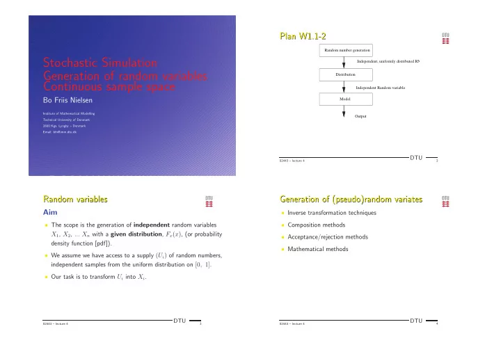
Plan W1.1-2 Plan W1.1-2

Random number generation Independent Random variable Output Independent, uniformly distributed RN Model Distribution

02443 – lecture 4 3

DTU

Random variables Random variables

Aim

• The scope is the generation of independent random variables

X1, X2, ... Xn with a given distribution, Fx(x), (or probability density function [pdf]).

• We assume we have access to a supply (Ui) of random numbers,

independent samples from the uniform distribution on [0, 1].

• Our task is to transform Ui into Xi.

02443 – lecture 4 4

DTU

Generation of (pseudo)random variates Generation of (pseudo)random variates

• Inverse transformation techniques
• Composition methods
• Acceptance/rejection methods
• Mathematical methods

02443 – lecture 4 5

DTU

Uniform distribution I Uniform distribution I

Our norm distribution or building brick, U(0, 1) f(x) = 1 F(x) = x for 0 ≤ x ≤ 1

1 1

Ex = 1

2

Vx =

1 12

02443 – lecture 4 6

DTU

Inverse transformation Inverse transformation

The cumulative distribution function (CDF) F(x) = P

• X ≤ x
• x

x F(x) x F(x) = P(X<=x) 02443 – lecture 4 7

DTU

The random variable F(X) The random variable F(X)

X F(X) X F(X) = U 02443 – lecture 4 8

DTU

From U to X From U to X

U * U = F(X) * U = F(X) * X = F (U)

−1

02443 – lecture 4 9

DTU

Inversion method Inversion method

The random variable U = F(X)

U=F(X) X

U = F(X) Fu(u) = P

• U ≤ u
• Fu(u) = P
• F(X) ≤ u
• = P
• X ≤ F −1(u)
• = F(F −1(u)) = u

I.e. F(X) is uniformly distributed.

02443 – lecture 4 10

DTU

Inversion method Inversion method

Assuming C1 functions (also for g and g−1) and let: X = g(Y ) Y : FY (y) = P

• Y ≤ y
• then

Fx(x) = P

• X ≤ x
• = P
• g(Y ) ≤ x
• = P
• Y ≤ g−1(x)
• = Fy(g−1(x))

If Y = U then Fu(u) = u, and Fx(x) = g−1(x). If X = F −1(U) then X will have the cdf F(x).

02443 – lecture 4 11

DTU

Uniform distribution II Uniform distribution II

Now, focus on U(a, b). f(x) = 1 b − a a ≤ x ≤ b F(x) = x − a b − a F −1(u) = a + (b − a)u X = a + (b − a)U ∈ U(a, b)

02443 – lecture 4 12

DTU

Exponential distribution Exponential distribution

The time between events in a Poisson process is exponential distribu-

• ted. (Arrival time)

F(x) = 1 − exp(−λx) EX = 1 λ F −1(u) = −1 λlog(1 − u) So (both 1 − U and U is uniform distributed) X = −log(U) λ ∈ Ex(λ)

02443 – lecture 4 13

DTU

Pareto Pareto

Is often used in connection to description of income (over a certain level). X ∈ Pa(k, β) F(x) = 1 − β x k x ≥ β X = β

• U − 1

k

• EX =

k k − 1β VX = k (k − 1)2(k − 2)β2 k > 1, 2

Pareto with X ≥ 0 F(x) = 1−

• 1 + x

β −k X = β

• U − 1

k − 1

• 02443 – lecture 4

14

DTU

Gaussian Gaussian

X a result of many (∞) independent sources (Central limit theorem) X ∈ N(µ, σ2) G ∈ N(0, 1) X = µ + σG G = Φ−1(U)

02443 – lecture 4 15

DTU

Mathematical Method Mathematical Method

• By means of transformation and other techniques we can obtain

stochastic variable with a certain distribution.

The Box-Muller method A transformation from polar

(θ = 2πU2, r =

• −2ln(U1)) into Cartesian

coordinates (X = G1 and Y = G2).   G1 G2   =

• −2ln(U1)

  cos(2πU2) sin(2πU2)   G1, G2 ∈ N0, 1

Central limit theorem

G =

n

• i=1

Ui − n 2

• eg. n = 6

02443 – lecture 4 16

DTU

Generation of cos and sin Generation of cos and sin

Sine and cosine can be calculated by the following acceptance/rejection algorith m:

• 1. Generate V1, V2 ∈ U(0, 1)
• 2. Generate R2 = V 2

1 + V 2 2

• 3. If R2 > 1 goto 1.
• 4. cos (2πU2) = V1

R , sin (2πU2) = V2 R

02443 – lecture 4 17

DTU

LN(α, β2) LN(α, β2)

Logarithmic Gaussian, LN(α, β2)

Y ∈ LN(α, β2) ln(Y ) ∈ Nα, β2 Y = exp(X) X = α + β G G ∈ N(0, 1)

02443 – lecture 4 18

DTU

General and mulitvariate normal distribution General and mulitvariate normal distribution

• Generate n independent values from an N(0, 1)

distribution,Zi inN(0, 1).

• Xi = µi + i

j=1 cijZj

• Where cij are the elements in the Cholesky factorisation of

Σ, Σ = CC′

02443 – lecture 4 19

DTU

Composition methods - hyperexponential distribution Composition methods - hyperexponential distribution

F(x) = 1 −

m

• i=1

pie−λix =

m

• i=1

pi

• 1 − e−λix

Formally we can express Z = XI where I ∈ {1, 2, . . . , m} with P{I = i} = pi and XI ∈ exp (λI)

• 1. Choose I ∈ {1, 2, . . . , m} with probabilities pi’s
• 2. Z = − 1

λi log (U)

02443 – lecture 4 20

DTU

Composition methods - Erlang distribution Composition methods - Erlang distribution

• The Erlang distribution is a special case of the Gamma

distribution with integer valued shape parameter

• An Erlang distributed random variable can be interpreted as a

sum of independent exponential variables

• We can generate an Erlang-n distributed random variate by

adding n exponential random variates. Z ∈ Erln(λ) E(Z) = n λ V (Z) = n λ2 Z =

n

• i=1

Xi =

n

• i=1

−1 λ log (Ui) = −1 λ log (Πn

i=1Ui)

02443 – lecture 4 21

DTU

Composition methods II Composition methods II

Generalization: f(x) =

• f(x|y)f(y)dy

X|Y : f(x|y) Y : f(y) Y is typical a parameter (eg. X|µ ∈ N(µ, σ2)) Generate:

• Generate Y from f(y).
• Generate X from f(x|y) where Y is used.

02443 – lecture 4 22

DTU

Acceptance/rejection Acceptance/rejection

Problem: we would like to generate X from pdf f, but it is much faster to generate Y with pdf g. NB. X and Y have the same sample space. If f(y) g(y) ≤ c for all y and some c

• Step 1. Generate Y having density g.
• Step 2. Generate a random number U
• If U ≤ f(Y )

cg(Y ) set X = Y .Otherwise return to step 1.

g(y)dy f(y) cg(y) = f(y)dy c

02443 – lecture 4 23

DTU Statistics Toolbox Version 4.0 (R13) 20-Jun-2002 . . . Random Number Generators. betarnd

• Beta random numbers.

binornd

• Binomial random numbers.

chi2rnd

• Chi square random numbers.

exprnd

• Exponential random numbers.

frnd

• F random numbers.

gamrnd

• Gamma random numbers.

geornd

• Geometric random numbers.

hygernd

• Hypergeometric random numbers.

iwishrnd

• Inverse Wishart random matrix.

lognrnd

• Lognormal random numbers.

Exercise 3 Exercise 3

• Generate simulated values from the following distributions

⋄ Exponential distribution ⋄ Normal distribution ⋄ Pareto distribution, with β = 1 and experiment with different values of k values: k = 2.05, k = 2.5, k = 3 og k = 4.

• Verify the results by comparing histograms with analytical

results.

• For the Pareto distribution compare mean value and variance,

with analytical results, which can be calculated as E{X} = β

k k−1 (for k > 1) and V ar{X} = β2 k (k−1)2(k−2) (for

k > 2)

02443 – lecture 4 25

DTU

Exercise 3 continued Exercise 3 continued

• For the normal distribution generate 100 95% confidence

intervals for the mean and variance based on 10 observations. Discuss the results.