Statistical Models & Computing Methods Lecture 1: Introduction - PowerPoint PPT Presentation

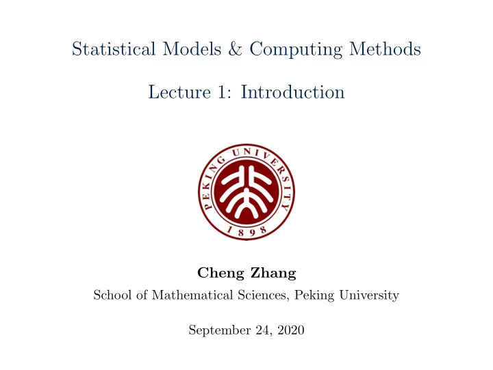
Statistical Models & Computing Methods Lecture 1: Introduction Cheng Zhang School of Mathematical Sciences, Peking University September 24, 2020

General Information 2/56 ◮ Class times: ◮ Thursday 6:40-9:30pm ◮ Classroom Building No.2, Room 401 ◮ Instructor: ◮ Cheng Zhang: chengzhang@math.pku.edu.cn ◮ Teaching assistants: ◮ Dequan Ye: 1801213981@pku.edu.cn ◮ Zihao Shao: zh.s@pku.edu.cn ◮ Tentative office hours: ◮ 1279 Science Building No.1 ◮ Thursday 3:00-5:00pm or by appointment ◮ Website: https://zcrabbit.github.io/courses/smcm-f20.html

Computational Statistics/Statistical Computing 3/56 ◮ A branch of mathematical sciences focusing on efficient numerical methods for statistically formulated problems ◮ The focus lies on computer intensive statistical methods and efficient modern statistical models. ◮ Developing rapidly, leading to a broader concept of computing that combines the theories and techniques from many fields within the context of statistics, mathematics and computer sciences.

Goals 4/56 ◮ Become familiar with a variety of modern computational statistical techniques and knows more about the role of computation as a tool of discovery ◮ Develop a deeper understanding of the mathematical theory of computational statistical approaches and statistical modeling. ◮ Understand what makes a good model for data. ◮ Be able to analyze datasets using a modern programming language (e.g., python).

Textbook 5/56 ◮ No specific textbook required for this course ◮ Recommended textbooks: ◮ Givens, G. H. and Hoeting, J. A. (2005) Computational Statistics, 2nd Edition, Wiley-Interscience. ◮ Gelman, A., Carlin, J., Stern, H., and Rubin, D. (2003). Bayesian Data Analysis, 2nd Edition, Chapman & Hall. ◮ Liu, J. (2001). Monte Carlo Strategies in Scientific Computing, Springer-Verlag. ◮ Lange, K. (2002). Numerical Analysis for Statisticians, Springer-Verlag, 2nd Edition. ◮ Hastie, T., Tibshirani, R. and Friedman, J. (2009). The Elements of Statistical Learning, 2nd Edition, Springer. ◮ Goodfellow, I., Bengio, Y. and Courville, A. (2016). Deep Learning, MIT Press.

Tentative Topics 6/56 ◮ Optimization Methods ◮ Gradient Methods ◮ Expectation Maximization ◮ Approximate Bayesian Inference Methods ◮ Markov chain Monte Carlo ◮ Variational Inference ◮ Scalable Approaches ◮ Applications in Machine Learning & Related Fields ◮ Variational Autoencoder ◮ Generative Adversarial Networks ◮ Flow-based Generative Models ◮ Bayesian Phylogenetic Inference

Prerequisites 7/56 Familiar with at least one programming language (with python preferred!). ◮ All class assignments will be in python (and use numpy). ◮ You can find a good Python tutorial at http://www.scipy-lectures.org/ You may find a shorter python+numpy tutorial useful at http://cs231n.github.io/python-numpy-tutorial/ Familiar with the following subjects ◮ Probability and Statistical Inference ◮ Stochastic Processes

Grading Policy 8/56 ◮ 4 Problem Sets: 4 × 15% = 60% ◮ Final Course Project: 40% ◮ up to 4 people for each team ◮ Teams should be formed by the end of week 4 ◮ Midterm proposal: 5% ◮ Oral presentation: 10% ◮ Final write-up: 25% ◮ Late policy ◮ 7 free late days, use them in your ways ◮ Afterward, 25% off per late day ◮ Not accepted after 3 late days per PS ◮ Does not apply to Final Course Project ◮ Collaboration policy ◮ Finish your work independently, verbal discussion allowed

Final Project 9/56 ◮ Structure your project exploration around a general problem type, algorithm, or data set, but should explore around your problem, testing thoroughly or comparing to alternatives. ◮ Present a project proposal that briefly describe your teams’ project concept and goals in one slide in class on 11/12. ◮ There will be in class project presentation at the end of the term. Not presenting your projects will be taken as voluntarily giving up the opportunity for the final write-ups. ◮ Turn in a write-up ( < 10 pages) describing your project and its outcomes, similar to a research-level publication.

Today’s Agenda 10/56 ◮ A brief overview of statistical approaches ◮ Basic concepts in statistical computing ◮ Convex optimization

Statistical Pipeline 11/56 Knowledge Data

Statistical Pipeline 11/56 Data

Statistical Pipeline 11/56 Knowledge Data D

Statistical Pipeline 11/56 Linear Models Latent Variable Models Neural Networks Bayesian Nonparametric Models Generalized Linear Models Knowledge Data Model D

Statistical Pipeline 11/56 Knowledge Data Model D p ( D| θ )

Statistical Pipeline 11/56 Gradient Descent EM Knowledge Data Model Inference MCMC D p ( D| θ ) Variational Methods

Statistical Pipeline 11/56 Gradient Descent EM Knowledge Data Model Inference MCMC D p ( D| θ ) Variational Methods

Statistical Pipeline 11/56 Gradient Descent Our focus EM Knowledge Data Model Inference MCMC D p ( D| θ ) Variational Methods

Statistical Models 12/56 “All models are wrong, but some are useful.” George E. P. Box Models are used to describe the data generating process, hence prescribe the probabilities of the observed data D p ( D| θ ) also known as the likelihood .

Examples: Linear Models 13/56 Data : D = { ( x i , y i ) } n i =1 Model : Y = Xθ + ǫ, ǫ ∼ N (0 , σ 2 I n ) ⇒ Y ∼ N ( Xθ, σ 2 I n ) −� Y − Xθ � 2 � � p ( Y | X, θ ) = (2 πσ 2 ) − n/ 2 exp 2 2 σ 2

Examples: Logistic Regression 14/56 Data : D = { ( x i , y i ) } n i =1 , y i ∈ { 0 , 1 } Model : Y ∼ Bernoulli( p ) 1 p = 1 + exp( − Xθ ) n p y i � i (1 − p i ) 1 − y i p ( Y | X, θ ) = i =1

Examples: Gaussian Mixture Model 15/56 Data : D = { y i } n i =1 , y i ∈ R d Model : y | Z = z ∼ N ( µ z , σ 2 z I d ) Z ∼ Categorical( α ) n K −� y i − µ k � 2 � � k ) ( − d/ 2) exp � � α k (2 πσ 2 2 p ( Y | µ, σ, α ) = 2 σ 2 k i =1 k =1

Examples: Phylogenetic Model 16/56

Examples: Phylogenetic Model 16/56 Data : DNA sequences D = { y i } n i =1

Examples: Phylogenetic Model 16/56 Data : DNA sequences D = { y i } n i =1

Examples: Phylogenetic Model 16/56 Data : DNA sequences D = { y i } n A i =1 A Model : Phylogenetic tree: ( τ, q ). G Substitution model: T ◮ stationary distribution: η ( a ρ ). A ◮ transition probability: C p ( a u → a v | q uv ) = P a u a v ( q uv ) C

Examples: Phylogenetic Model 16/56 Data : DNA sequences D = { y i } n AT · · · i =1 Model : Phylogenetic tree: ( τ, q ). GG · · · Substitution model: ◮ stationary distribution: η ( a ρ ). ◮ transition probability: AC · · · p ( a u → a v | q uv ) = P a u a v ( q uv ) CC · · · n � � η ( a i � p ( Y | τ, q ) = ρ ) v ( q uv ) P a i u a i i =1 a i ( u,v ) ∈ E ( τ )

Examples: Phylogenetic Model 16/56 Data : DNA sequences D = { y i } n AT · · · i =1 Model : Phylogenetic tree: ( τ, q ). GG · · · Substitution model: ◮ stationary distribution: η ( a ρ ). ◮ transition probability: AC · · · p ( a u → a v | q uv ) = P a u a v ( q uv ) CC · · · n � � η ( a i � p ( Y | τ, q ) = ρ ) v ( q uv ) P a i u a i i =1 a i ( u,v ) ∈ E ( τ ) where a i agree with y i at the tips

Examples: Latent Dirichlet Allocation 17/56 ◮ Each topic is a distribution over words ◮ Documents exhibit multiple topics

Examples: Latent Dirichlet Allocation 17/56 Data : a corpus D = { w i } M i =1 Model : for each document w in D ,

Examples: Latent Dirichlet Allocation 17/56 Data : a corpus D = { w i } M i =1 Model : for each document w in D , ◮ choose a mixture of topics θ ∼ Dir( α )

Examples: Latent Dirichlet Allocation 17/56 Data : a corpus D = { w i } M i =1 Model : for each document w in D , ◮ choose a mixture of topics θ ∼ Dir( α ) ◮ for each of the N words w n , z n ∼ Multinomial( θ ) , w n | z n , β ∼ p ( w n | z n , β )

Examples: Latent Dirichlet Allocation 17/56 Data : a corpus D = { w i } M i =1 Model : for each document w in D , ◮ choose a mixture of topics θ ∼ Dir( α ) ◮ for each of the N words w n , z n ∼ Multinomial( θ ) , w n | z n , β ∼ p ( w n | z n , β ) M N d � � � � p ( D| α, β ) = p ( θ d | α ) p ( z dn | θ d ) p ( w dn | z dn , β ) dθ d d =1 n =1 z dn

Exponential Family 18/56 Many well-known distributions take the following form p ( y | θ ) = h ( y ) exp ( φ ( θ ) · T ( y ) − A ( θ )) ◮ φ ( θ ): natural/canonical parameters ◮ T ( y ): sufficient statistics ◮ A ( θ ): log-partition function �� � A ( θ ) = log h ( y ) exp( φ ( θ ) · T ( y )) dy y

Examples: Bernoulli Distribution 19/56 Y ∼ Bernoulli( θ ): p ( y | θ ) = θ y (1 − θ ) 1 − y � � � � θ = exp log y + log(1 − θ ) 1 − θ � � θ ◮ φ ( θ ) = log 1 − θ ◮ T ( y ) = y ◮ A ( θ ) = − log(1 − θ ) = log(1 + e φ ( θ ) ) ◮ h ( y ) = 1

Examples: Gaussian Distribution 20/56 Y ∼ N ( µ, σ 2 ): 1 � − 1 � p ( y | µ, σ 2 ) = 2 σ 2 ( y − µ ) 2 √ 2 πσ exp � µ 2 σ 2 y 2 − µ 2 1 1 � = √ 2 π exp σ 2 y − 2 σ 2 − log σ ◮ φ ( θ ) = [ µ σ 2 , − 1 2 σ 2 ] T ◮ T ( y ) = [ y, y 2 ] T ◮ A ( θ ) = µ 2 2 σ 2 + log σ 1 ◮ h ( y ) = √ 2 π