Statistical Geometry Processing Winter Semester 2011/2012 Linear - - PowerPoint PPT Presentation

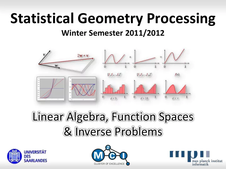
Statistical Geometry Processing

Winter Semester 2011/2012

Linear Algebra, Function Spaces & Inverse Problems

Vector and Function Spaces

3

Vectors

vectors are arrows in space classically: 2 or 3 dim. Euclidian space

4

Vector Operations

v w v + w “Adding” Vectors: Concatenation

5

Vector Operations

v Scalar Multiplication: Scaling vectors (incl. mirroring) 1.5·v 2.0·v

• 1.0·v

6

You can combine it...

v Linear Combinations: This is basically all you can do. w 2w + v







n i i i 1

v r 

7

Vector Spaces

Vector space:

• Set of vectors V
• Based on field F (we use only F = )
• Two operations:
• Adding vectors u = v + w (u, v, w  V)
• Scaling vectors w = v (u  V,   F)
• Vector space axioms:

8

Additional Tools

More concepts:

• Subspaces, linear spans, bases
• Scalar product
• Angle, length, orthogonality
• Gram-Schmidt orthogonalization
• Cross product (ℝ3)
• Linear maps
• Matrices
• Eigenvalues & eigenvectors
• Quadratic forms

(Check your old math books)

9

Example Spaces

Function spaces:

• Space of all functions f:   
• Space of all smooth Ck functions f:   
• Space of all functions f: [0..1]5  8
• etc...

1 1 1

+ =

10

Function Spaces

Intuition:

• Start with a finite dimensional vector
• Increase sampling density towards infinity
• Real numbers: uncountable amount of dimensions

1 1 1 d = 9 d = 18 d =  [f1,f2,...,f9]T [f1,f2,...,f18]T f(x)

11

Dot Product on Function Spaces

Scalar products

• For square-integrable functions f, g:   n  , the

standard scalar product is defined as:

• It measures an abstract norm and “angle” between

function (not in a geometric sense)

• Orthogonal functions:
• Do not influence each other in linear combinations.
• Adding one to the other does not change the value in the other
• nes direction.





  dx x g x f g f ) ( ) ( :

12

Approximation of Function Spaces

Finite dimensional subspaces:

• Function spaces with infinite dimension are hard to

represented on a computer

• For numerical purpose, finite-dimensional subspaces are

used to approximate the larger space

• Two basic approaches

13

Approximation of Function Spaces

Task:

• Given: Infinite-dimensional function space V.
• Task: Find f  V with a certain property.

Recipe: “Finite Differences”

• Sample function f on discrete grid
• Approximate property discretely
• Derivatives => finite differences
• Integrals => Finite sums
• Optimization: Find best discrete function

14

Recipe: “Finite Elements”

• Choose basis functions b1, ..., bd  V
• Find 𝑔

= 𝜇𝑗𝑐𝑗

𝑒 𝑗=1

that matches the property best

• 𝑔

is described by (1,...,d)

Approximation of Function Spaces

actual solution function space basis approximate solution

15

Examples

0,2 0,4 0,6 0,8 1 1,2 1,4 1,6 1,8 2

0,5 1 1,5 2

Monomial basis

• 1,5
• 1
• 0,5

0,5 1 1,5 2

0,5 1 1,5 2

Fourier basis

 2

B-spline basis, Gaussian basis

16

“Best Match”

Linear combination matches best

• Solution 1: Least squares minimization

𝑔 𝑦 − 𝜇𝑗𝑐𝑗 𝑦

𝑜 𝑗=1 2

𝑒𝑦 → 𝑛𝑗𝑜

ℝ

• Solution 2: Galerkin method

∀𝑗 = 1. . 𝑜: 𝑔 − 𝜇𝑗𝑐𝑗

𝑜 𝑗=1

, 𝑐𝑗 = 0

• Both are equivalent

17

Optimality Criterion

Given:

• Subspace W ⊆ V
• An element 𝐰 ∈ V

Then we get:

• 𝐱 ∈ W minimizes the quadratic error w − 𝐰 2

(i.e. the Euclidean distance) if and only if:

• the residual w − 𝐰 is orthogonal to W

Least squares = minimal Euclidean distance W V

𝐰 𝐱

18

Formal Derivation

Least-squares

E 𝑔 = 𝑔 𝑦 − 𝜇𝑗𝑐𝑗 𝑦

𝑜 𝑗=1 2

𝑒𝑦

ℝ

= 𝑔2 𝑦 − 2 𝜇𝑗𝑔 𝑦 𝑐𝑗 𝑦 + 𝜇𝑗

𝑜 𝑗=1

𝜇𝑘𝑐𝑗 𝑦 𝑐

𝑘 𝑦 𝑜 𝑗=1 𝑜 𝑗=1

𝑒𝑦

ℝ

Setting derivatives to zero:

𝛼E 𝑔 = −2 𝜇1 𝑔, 𝑐1 ⋮ 𝜇𝑜 𝑔, 𝑐𝑜 + 𝜇1, … , 𝜇𝑜 ⋱ ⋮ ⋰ ⋯ 𝑐𝑗 𝑦 , 𝑐

𝑘 𝑦

⋯ ⋰ ⋮ ⋱

Result:

∀𝑘 = 1. . 𝑜: 𝑔 − 𝜇𝑗𝑐𝑗

𝑜 𝑗=1

, 𝑐

𝑘 = 0

Linear Maps

20

Linear Maps

A Function

• f: V  W between vector spaces V, W

is linear if and only if:

• v1,v2V:

f (v1+v2) = f (v1) + f (v2)

• vV, F: f (v) = f (v)

Constructing linear mappings:

A linear map is uniquely determined if we specify a mapping value for each basis vector of V.

21

Matrix Representation

Finite dimensional spaces

• Linear maps can be represented as matrices
• For each basis vector vi of V, we specify the mapped

vector wi.

• Then, the map f is given by:

n n n

v v v v f f w w v                         ... ) (

1 1 1



22

Matrix Representation

This can be written as matrix-vector product:

The columns are the images of the basis vectors (for which the coordinates of v are given)

                     

n n

v v v f  

1 1

| | | | ) ( w w

23

Linear Systems of Equations

Problem: Invert an affine map

• Given: Mx = b
• We know M, b
• Looking for x

Solution

• Set of solutions: always an affine subspace of n,
• r the empty set.
• Point, line, plane, hyperplane...
• Innumerous algorithms for solving linear systems

24

Solvers for Linear Systems

Algorithms for solving linear systems of equations:

• Gaussian elimination: O(n3) operations for n  n matrices
• We can do better, in particular for special cases:
• Band matrices:

constant bandwidth

• Sparse matrices:

constant number of non-zero entries per row

– Store only non-zero entries – Instead of (3.5, 0, 0, 0, 7, 0, 0),

store [(1:3.5), (5:7)]

25

Solvers for Linear Systems

Algorithms for solving linear systems of n equations:

• Band matrices, O(1) bandwidth:
• Modified O(n) elimination algorithm.
• Iterative Gauss-Seidel solver
• converges for diagonally dominant matrices
• Typically: O(n) iterations, each costs O(n) for a sparse matrix.
• Conjugate Gradient solver
• Only symmetric, positive definite matrices
• Guaranteed: O(n) iterations
• Typically good solution after O( n) iterations.

More details on iterative solvers: J. R. Shewchuk: An Introduction to the Conjugate Gradient Method Without the Agonizing Pain, 1994.

26

Eigenvectors & Eigenvalues

Definition:

• Linear map M, non-zero vector x with

Mx = x

•  an is eigenvalue of M
• x is the corresponding eigenvector.

27

Example

Intuition:

• In the direction of an eigenvector, the linear map acts like

a scaling

• Example: two eigenvalues (0.5 and 2)
• Two eigenvectors
• Standard basis contains no eigenvectors



28

Eigenvectors & Eigenvalues

Diagonalization:

In case an n  n matrix M has n linear independent eigenvectors, we can diagonalize M by transforming to this coordinate system: M = TDT-1.

29

Spectral Theorem

Spectral Theorem:

If M is a symmetric n  n matrix of real numbers (i.e. M = MT), there exists an orthogonal set of n eigenvectors. This means, every (real) symmetric matrix can be diagonalized: M = TDTT with an orthogonal matrix T.

30

Computation

Simple algorithm

• “Power iteration” for symmetric matrices
• Computes largest eigenvalue even for large matrices
• Algorithm:
• Start with a random vector (maybe multiple tries)
• Repeatedly multiply with matrix
• Normalize vector after each step
• Repeat until ration before / after normalization converges

(this is the eigenvalue)

• Intuition:
• Largest eigenvalue = “dominant” component/direction

31

Powers of Matrices

What happens:

• A symmetric matrix can be written as:
• Taking it to the k-th power yields:
• Bottom line: Eigenvalue analysis key to understanding

powers of matrices.

T 1 T

T T TDT M            

n

  

T 1 T T T T

... T T T TD TDT TDT TDT M               

k n k k k

  

32

Improvements

Improvements to the power method:

• Find smallest? – use inverse matrix.
• Find all (for a symmetric matrix)? – run repeatedly,
• rthogonalize current estimate to already known

eigenvectors in each iteration (Gram Schmidt)

• How long does it take? – ratio to next smaller eigenvalue,

gap increases exponentially.

There are more sophisticated algorithms based on this idea.

33

Generalization: SVD

Singular value decomposition:

• Let M be an arbitrary real matrix (may be rectangular)
• Then M can be written as:
• M = U D VT
• The matrices U, V are orthogonal
• D is a diagonal matrix (might contain zeros)
• The diagonal entries are called singular values.
• U and V are different in general. For diagonalizable

matrices, they are the same, and the singular values are the eigenvalues.

34

M U D VT

Singular Value Decomposition

Singular value decomposition

1 2 3 4

=

    

• rthogonal

    

• rthogonal

35

Singular Value Decomposition

Singular value decomposition

• Can be used to solve linear systems of equations
• For full rank, square M:

M = U D VT  M-1 = (U D VT)-1 = (VT)-1 D-1 (U-1) = V D-1 UT

• Good numerical properties (numerically stable)
• More expensive than iterative solvers
• The OpenCV library provides a very good implementation
• f the SVD

Linear Inverse Problems

37

Inverse Problems

Settings

• A (physical) process f takes place
• It transforms the original input x into an output b
• Task: recover x from b

Examples:

• 3D structure from photographs
• Tomography: values from line integrals
• 3D geometry from a noisy 3D scan

38

Linear Inverse Problems

Assumption: f is linear and finite dimensional

f (x) = b  Mf x = b

Inversion of f is said to be an ill-posed problem, if one

• f the following three conditions hold:
• There is no solution
• There is more than one solution
• There is exactly one solution, but the SVD contains very

small singular values.

39

Ill posed Problems

Ratio: Small singular values amplify errors

• Assume inexact input
• Measurement noise
• Numerical noise
• Reminder: M-1 = V D-1 UT
• Orthogonal transforms preserve norm of x,

so V and U do not cause problems

does not hurt (orthogonal) does not hurt (orthogonal) this one is decisive

40

Ill posed Problems

Ratio: Small singular values amplify errors

• Reminder: x = M-1b = (V D-1 UT)b
• Say D looks like that:
• Any input noise in b in the direction of the fourth right

singular vector will be amplified by 109.

• If our measurement precision is less than that, the result

will be unusable.

• Does not depend on how we invert the matrix.
• Condition number: max /min

          

000000001 . 9 . 1 . 1 5 . 2

: D

41

Ill Posed Problems

Two problems:

(1) Mapping destroys information

• goes below noise level
• cannot be recovered by any means

(2) Inverse mapping amplifies noise

• yields garbage solution
• even remaining information not recovered
• extremely large random solutions are obtained

We can do something about problem #2

          

000000001 . 9 . 1 . 1 5 . 2

: D

42

Regularization

Regularization

• Avoiding destructive noise caused by inversion
• Various techniques
• Goal: ignore the misleading information
• Subspace inversion:
• Ignore subspace with small singular values

– needs an SVD, risk of ringing

• Additional assumptions:

– smoothness (or something similar) – make compound problem (f -1 + assumptions) well posed

• We will look at this in detail later

43

Illustration of the Problem

• riginal function

smoothed function f g f ⊗ g

forward problem

44

Illustration of the Problem

f’ f ⊗ g

inverse problem

smoothed function reconstructed function

45

Illustration of the Problem

f’ f ⊗ g

inverse problem

regularized reconstructed function smoothed function

46

Illustration of the Problem

• riginal function

f g Frequency Domain G Frequency Domain G-1

regularization

47 1.4 1.5 0.8 0.9 1.3 0.8 0.7 

            

1.2 1.5 0.3 0.4 1.6 0.2 0.3 

                          

Illustration of the Problem

• riginal function

smoothed function f g f ⊗ g

2 1 1 1 2 1 1 2 1 1 2 1 1 2 1 1 2 1 1 1 2

*

forward problem

=

1 3

48 1.4 1.5 0.8 0.9 1.2 0.8 0.7 

            

1.2 1.5 0.3 0.4 1.6 0.2 0.3 1.4 1.5 0.8 0.9 1.3 0.8 0.7 

                          

Illustration of the Problem

• riginal function

smoothed function f g f ⊗ g

2 1 1 1 2 1 1 2 1 1 2 1 1 2 1 1 2 1 1 1 2

*

forward problem

=

3

• 1

             

solution (from 2 digits) correct

49

Analysis

              2

1 1 1 2 1 1 2 1 1 2 1 1 2 1 1 2 1 1 1 2

Matrix Spectrum Dominant Eigenvectors Smallest Eigenvectors

• 0,6
• 0,4
• 0,2

0,2 0,4 0,6 1 2 3 4 5 6 7 0,2 0,2 1 2 3 4 5 6 7 4 3,2 3,2 0,2 0,4 0,6 0,8 1 1,2 1,4 1 2 3 4 5 6 7

• 0,6
• 0,4
• 0,2

0,2 0,4 0,6

50

Digging Deeper...

Let’s look at this example again:

• Convolution operation:

𝑔′(𝑦) = 𝑔(𝑢) ∙ 𝑕 𝑢 − 𝑦 𝑒𝑢

ℝ

• Shift-invariant linear operator

f g

              2

1 1 1 2 1 1 2 1 1 2 1 1 2 1 1 2 1 1 1 2

continuous discrete

51

Convolution Theorem

Fourier Transform

• Function space:

𝑔: 0. . 2π → ℝ (suff. smooth)

• Fourier basis:

1, cos 𝑙𝑦 , sin 𝑙𝑦|𝑙 = 1,2, …

• Properties
• The Fourier basis is an orthogonal basis (standard scalar prod.)
• The Fourier basis diagonalizes all shift-invariant linear operators

52

Convolution Theorem

This means:

• Let 𝐺: ℕ → ℝ be the Fourier transform (FT) of

𝑔: [0. . 2π] → ℝ

• Then: 𝑔 ⨂ 𝑕 = 𝐺𝑈−1(𝐺 ⋅ 𝐻)

Consequences

• Fourier spectrum of convolution operator (“filter”)

determines well-posedness of inverse operation (deconvolution)

• Certain frequencies might be lost
• In our example: high frequencies

Quadratic Forms

54

Multivariate Polynomials

A multi-variate polynomial of total degree d:

• A function f: n  , x  f(x)
• f is a polynomial in the components of x
• Any 1D direction f(s + tr) is a polynomial of

maximum degree d in t.

Examples:

• f(x, y) := x + xy + y is of total degree 2. In diagonal

direction, we obtain f(t[1/ 2, 1/ 2]T) = t2.

• f(x, y) := c20x2 + c02y2 + c11xy + c10x + c01y + c00 is a

quadratic polynomial in two variables

55

Quadratic Polynomials

In general, any quadratic polynomial in n variables can be written as:

• xTA x + bTx + c
• A is an n  n matrix, b is an n-dim. vector, c is a number
• Matrix A can always be chosen to be symmetric
• If it isn’t, we can substitute by 0.5·(A + AT), not changing

the polynomial

56

Example

Example:

x x x x x x x                                                                                                    4 5 . 2 5 . 2 1 4 2 3 1 4 3 2 1 2 1 4 ) 5 . 2 5 . 2 ( 1 4 ) 3 2 ( 1 4 3 2 1 4 3 2 1 ] [ 4 3 2 1 ] [ 4 3 2 1 ) (

T T 2 2 2 2 T

y xy x y xy x y y x y y x x x y x y x y x y x y x f y x f

57

Quadratic Polynomials

Specifying quadratic polynomials:

• xTA x + bTx + c
• b shifts the function in space (if A has full rank):
• c is an additive constant

     

c x x c x x x x c x x                        x A A A A A A 2

T sym.) (A T T T T

= b

58

Some Properties

Important properties

• Multivariate polynomials form a vector space
• We can add them component-wise:

2x2 + 3y2 + 4xy + 2x + 2y + 4 + 3x2 + 2y2 + 1xy + 5x + 5y + 5 = 5x2 + 5y2 + 5xy + 7x + 7y + 9

• In vector notation:

xTA1 x + b1

Tx + c1

+ (xTA2x + b2

Tx + c2)

= xT(A1 + A2)x + (b1 + b2)Tx + (c1 + c2)

59

Quadratic Polynomials

Quadrics

• Zero level set of a quadratic polynomial: “quadric”
• Shape depends on eigenvalues of A
• b shifts the object in space
• c sets the level

60

Shapes of Quadrics

Shape analysis:

• A is symmetric
• A can be diagonalized with orthogonal eigenvectors
• Q contains the principal axis of the quadric
• The eigenvalues determine the quadratic growth

(up, down, speed of growth)    

x x x x

n n

Q Q Q Q Ax x                              

  1 T 1 T T T

61

Shapes of Quadratic Polynomials

1 = 1, 2 = 1 1 = 1, 2 = -1 1 = 1, 2 = 0

62

The Iso-Lines: Quadrics

1 > 0, 2 > 0 1 < 0, 2 > 0 elliptic hyperbolic 1 = 0, 2  0 degenerate case

63

Quadratic Optimization

Quadratic Optimization

• Minimize quadratic objective function

xTA x + bTx + c

• Required: A > 0 (only positive eigenvalues)
• It’s a paraboloid with a unique minimum
• The vertex (critical point) can be determined

by simply solving a linear system

• Necessary and sufficient condition

2A x = –b

64

Condition Number

How stable is the solution?

• Depends on Matrix A

good bad

65

Regularization

• Sums of positive semi-definite matrices are

positive semi-definite

• Add regularizing quadric
• “Fill in the valleys”
• Bias in the solution

Example

• Original:

xTA x + bTx + c

• Regularized: xT(A + I )x + bTx + c

Regularization

A + I

66

Rayleigh Quotient

Relation to eigenvalues:

• Min/max eigenvalues of a symmetric A expressed as

constraint quadratic optimization:

• The other way round – eigenvalues solve a certain type of

constrained, (non-convex) optimization problem.

 

Ax x x x Ax x

T 1 T T min

min min



 

x



 

Ax x x x Ax x

T 1 T T max

max max



 

x



67

Coordinate Transformations

One more interesting property:

• Given a positive definite symmetric (“SPD”) matrix M

(all eigenvalues positive)

• Such a matrix can always be written as square of another

matrix:

      

                      

n T T T

D D T D T D T T D D T   

1 2 T

TDT M

68

SPD Quadrics

Interpretation:

• Start with a unit positive quadric xTx.
• Scale the main axis (diagonal of D)
• Rotate to a different coordinate system (columns of T)
• Recovering main axis from M: Compute eigensystem

(“principal component analysis”)

 

2 T

D T   TDT M I Identity

main axis

x xT Mx xT

69

Why should I care?

What are quadrics good for?

• log-probability of Gaussian models
• Estimation in Gaussian probabilistic

models...

• ...is quadratic optimization.
• ...is solving of linear systems of equations.
• Quadratic optimization
• easy to use & solve
• feasible :-)
• Approximate more complex models locally

Gaussian normal distribution

 

          

2 2 ,

2 exp π 2 1 ) (   

 

x x p

Groups and Transformations

71

Groups

Definition: A set G with operation ⊗ is called a group (G, ⊗), iff:

• Closed:

⊗: 𝐻 × 𝐻 → 𝐻 (always maps back to G)

• Associativity:

(𝑔 ⊗ g) ⊗ ℎ = 𝑔 ⊗ (g ⊗ ℎ)

• Neutral element: there exists 𝑗𝑒 ∈ 𝐻 such that for any

𝑕 ∈ 𝐻: 𝑕 ⊗ 𝑗𝑒 = 𝑕

• Inverse element: For each 𝑕 ∈ 𝐻 there exists 𝑕−1 ∈ 𝐻

such that 𝑕 ⊗ 𝑕−1 = 𝑕−1 ⊗ 𝑕 = 𝑗𝑒

Abelian Groups

• The group is commutative iff always 𝑔 ⊗ g = 𝑕 ⊗ 𝑔

72

Examples of Groups

Examples:

• G = invertible matrices, ⊗ = composition (matrix mult.)
• G = invertible affine transformation of ℝ𝑒, ⊗ =

composition

(matrix form: homogeneos coordinates)

• G = bijections of a set S to itself, ⊗ = composition
• G = smooth Ck bijections of a set S to itself, ⊗ = composition
• G = global symmetry transforms of a shape, ⊗ = composition
• G = permutation of a discrete set, ⊗ = composition

73

Examples of Groups

Examples:

• G = invertible matrices, ⊗ = composition (matrix mult.)
• G = invertible affine transformation of ℝ𝑒

Subgroups:

• G = similarity transform (translation, rotation, mirroring,

scaling ≠ 0)

• E(d): G = rigid motions (translation, rotation, mirroring)
• SE(d): G = rigid motions (translation, rotation)
• O(d): G = orthogonal matrix (rotation, mirroring)

(columns/rows orthonormal)

• SO(d): G = orthogonal matrix (rotation)

(columns/rows orthonormal, determinant 1)

• G = translations (the only commutative group out of these)

74

Examples of Groups

Examples:

• G = global symmetry transforms of a 2D shape

75

Examples of Groups

Examples:

• G = global symmetry transforms of a 3D shape

(extended to infinity) (extended to infinity)

76

Outlook

More details on this later

• Symmetry groups
• Structural regularity
• Crystalographic groups and regular lattices