Statistical Discrimination, Employer Learning, and Employment - PowerPoint PPT Presentation

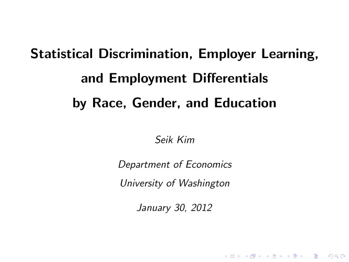
Statistical Discrimination, Employer Learning, and Employment Di¤erentials by Race, Gender, and Education Seik Kim Department of Economics University of Washington January 30, 2012

Imperfect Information I in hiring and wage-setting processes, employers make judgments about the value of workers using all information available at the time of making decisions. I however, the workers’ productivity is never perfectly observed, and employers must make predictions on the basis of limited information. I e.g., potential workers, at the time of labor market entry, do not have past labor market experience, and employers receive only noisy signals of worker productivity, such as cvs, recommendation letters, and interviews, as well as race, gender, and education.

Information and Screening Discrimination I in real world, it is possible that the same worker is evaluated di¤erently by di¤erent employers because ... I an employer’s ability to screen the productivity of a worker I depends on whether they share a similar cultural background e.g. they are from the same high school I depends on the worker’s race, gender, or education group e.g. two individuals of the same gender, education, and experience, but of di¤erent race I screening discrimination (Cornell and Welch, 1996) I employers’ belief: workers have the same ex ante productivity I employers’ ability to screen: worker-employer speci…c

Employer Learning and Information I employer learning hypothesis as young workers become experienced, past performance records become available to employers allowing them to make better predictions. I as employers learn about workers’ productivity, wages and employment opportunities will be a¤ected. I the theory of statistical discrimination, accompanied by the employer learning hypothesis, predicts that the degree of discrimination will decrease with the labor market experience of workers.

Tests for Statistical Discrimination I require some variables available to researchers be not observed by employers (Altonji and Pierret, 2001; Pinkston, 2006) I require employer-provided performance evaluation data (Neumark, 1999; Pinkston, 2003) I however, such variables are di¢cult to …nd in practice. I this paper develops a test that does NOT rely on those speci…c variables. I the data requirement for the proposed test is minimal cross-section on employment status, potential experience, and some variables on which discrimination is based, such as race, gender, and education.

Pros and Cons of Using Employment Opportunities I focus on employment opportunities rather than wage levels. discrimination will in‡uence the former more than the latter if the Equal Employment Opportunity Act prohibits wage di¤erences among workers performing the same task. I employment is measured as a binary variable. wage is continuous and contains more information.

Road Map I theory I statistical discrimination at labor market entry Aigner & Cain (1977), Lundberg & Startz (1983), Cornell & Welch (1996) I experience, employer learning, and statistical discrimination Altonji and Pierret (2001), Pinkston (2006) I testable implications I evidence I data: the March CPS for 1977-2010 I empirical …ndings I alternative explanations I concluding remarks

Basic Setting I employers announce job vacancies. receive and evaluate applications. may give o¤ers if the perceived productivity exceed their own pre-set productivity threshold. I potential workers apply for open positions, possibly more than one. no wage negotiation, but can choose if multiple o¤ers. I in the market a su¢ciently high signal is necessary for an o¤er, but does not guarantee an o¤er. if some o¤ers are turned down, employers may give o¤ers to other quali…ed candidates. some positions may remain un…lled and some applicants will remain unemployed.

Worker I a worker i is characterized by the productivity, P ij , at job j . P ij = r 0 X ij + r 0 j η i , (1) I vector X ij observed by both employers and researchers. e.g. labor market experience and possibly job tenure e.g. not necessarily race, gender, and/or education I vector η i consists of a …nite number of skill measures. may be observed by some employers, but not by researchers. has a multivariate normal distribution. I r is a vector of parameters common to all employers. I r j is an employer-speci…c non-random weight.

Employer I an employer j receives applications. makes predictions about the productivity of the applicants. I I ij : the set of information that employer j has about worker i at the time when worker i enters the labor market. I I ij is worker-employer speci…c includes X ij as well as race, gender, and education. may also include factors that are not observed by researchers and other employers. I worker i ’s productivity is perceived by employer j as E [ P ij j I ij ] = r 0 X ij + r 0 j E [ η i j I ij ] . (2) I di¤erent employers may rank the same applicant di¤erently.

Statistical Discrimination at Labor Market Entry I employers classify individuals into group A and group B. I employers believe that productivity is ex ante the same, but I i 2 A , j � I i 2 B , j , and I i 2 A , j 6 = I i 2 B , j for any j . (3) I (3) implies that the signals from group B workers are noisier than those from group A workers. I S ij : the signal that employer j receives from applicant i ’s η i . then, (3) can be represented as S i 2 A , j = r 0 j η i + ξ i 2 A , j and S i 2 B , j = r 0 j η i + ξ i 2 B , j , (4) � � 0 , σ 2 with σ 2 A ξ < σ 2 where ξ � N B ξ . ξ I use the common subscript i in (3) and (4) to emphasize the fact that the two workers are identical except for their group memberships.

Statistical Discrimination at Labor Market Entry I (3) and/or (4) imply � � �� > Var � � �� r 0 r 0 Var E j η i j I i 2 A , j E j η i j I i 2 B , j for any j . (5) I e.g. employer does not have any screening ability for B: � h i� r 0 E [ η i j I i 2 B , j ] = E [ η i ] ) Var E j η i j I i 2 B , j = 0. I e.g. employer perfectly observes the productivity of A: � h i� � � r 0 r 0 E [ η i j I i 2 A , j ] = η i ) Var E j η i j I i 2 A , j = Var j η i . I another way of deriving (5) is σ 2 η E [ P ij j I ij ] = E [ P ij j S ij , X ij ] = r 0 X ij + S ij , (6) σ 2 η + σ 2 ξ I (3), (4), and/or (5) imply that group B members are likely to be middle-ranked group A members tend to be top- or bottom-ranked

Statistical Discrimination at Labor Market Entry I since top-ranked applicants are more likely to get o¤ers, a group A member has a higher chance to get an initial o¤er. I the fact that group A members get more initial o¤ers does not necessarily imply a lower unemployment rate for group A than group B. I e.g. if all employers require the same skill and if they have an identical information set, all employers will rank all the applicants the same. group B unemployment rate < group A unemployment rate

Statistical Discrimination at Labor Market Entry I if employers require di¤erent skills and if information sets are heterogeneous, group B unemployment rate > group A unemployment rate Proposition 1. When employers statistically discriminate against group B workers in comparison to group A workers, the group B unemployment rate will be larger than the group A unemployment rate at the time of labor market entry.

Employer Learning and Statistical Discrimination I worker i accepts the o¤er from employer j . worker i produces an output, Q ijt , in each experience level t = 1 , 2 , ..., T . assume that there is no human capital accumulation. I q ijt is a proxy for r 0 j η i of the worker. Q ijt � r 0 X ij q ijt = r 0 = j η i + ε ijt , for t = 1 , 2 , ..., T , where ε ijt ’s are iid normal random variables with E [ ε i 2 A , t ] = E [ ε i 2 B , t ] = 0 and Var ( ε i 2 A , t ) = Var ( ε i 2 B , t ) = σ 2 ε and are independent of ξ ij .

Employer Learning and Statistical Discrimination I employer j observes q ij 1 , q ij 2 , ..., q ijT , in each period and subsequently updates his or her initial evaluation about r 0 j η i of the worker i . the proof below is similar to that in Pinkston (2006). E [ P ij j I ij , q ij 1 , ..., q ijT ] � � r 0 X ij + E r 0 j η i j r 0 j η i + ξ ij , r 0 j η i + ε ij 1 , ..., r 0 = j η i + ε ijT ! ξ ∑ T σ 2 σ 2 ε S ij + σ 2 t = 1 q ijt η r 0 X ij + = . (7) ε σ 2 T σ 2 σ 2 ξ + σ 2 σ 2 ξ η + ε T σ 2 ξ + σ 2 ε

Employer Learning and Statistical Discrimination I as workers become more experienced, employer j learns more about their productivity, and the distribution of evaluations approaches the true productivity distribution σ 4 η Var ( E [ P ij j I ij , q ij 1 , ..., q ijT ]) = σ 2 ε σ 2 ξ σ 2 η + T σ 2 ξ + σ 2 ε I the amount of learning is greater for B than A. σ 2 d 2 η > 0, d σ 2 σ 2 ε σ 2 ξ dT σ 2 ξ η + T σ 2 ξ + σ 2 ε