Starting from the next page, we provide the preprint version of our - - PDF document

▶

Aug 20, 2023 269 likes •427 views

1 Starting from the next page, we provide the preprint version of our following IEEE TKDE paper (Zhang et al. 2013). An extended abstract of our paper, in the same title, was also published in CIKM 2012. Nan Zhang, Chengkai Li, Naeemul Hassan,

SLIDE 1

Starting from the next page, we provide the preprint version of our following IEEE TKDE paper (Zhang et al. 2013). An extended abstract of our paper, in the same title, was also published in CIKM 2012. Nan Zhang, Chengkai Li, Naeemul Hassan, Sundaresan Rajasekaran, and Gautam Das. On Skyline Groups. IEEE Transactions

n Knowledge and Data Engineering, vol. 99, no. PrePrints, p. 1, 2013.

The following paper (Im and Park 2012) also studied the problem of computing skyline groups. Hyeonseung Im and Sungwoo Park. Group skyline computation. Information Sciences, volume 188, 1 April 2012, pages 151-169. We discovered this paper after we submitted the final version of the IEEE TKDE paper, which thus did not get to discuss this paper. Below we provide a brief comparison of (Zhang et al. 2013) and (Im and Park 2012). The differences are also summarized in the tables below. In (Im and Park 2012), the authors proposed two algorithms, GDynamic and GIncremental. GDynamic is based on dynamic programming and is only applicable for aggregate function SUM. In (Zhang et al. 2013), the OSM-based algorithm is applicable for SUM, MIN and MAX. It is similar to GDynamic. However, devising this algorithm for MIN/MAX was non-trivial, particularly because MIN/MAX, unlike SUM, are not strictly monotone in all arguments. This difference also required our OSM-based algorithm to identify unique skyline vectors instead of all skyline groups. GIncremental in (Im and Park 2012) is based on two properties which are special versions of the WCM property proposed in (Zhang et al. 2013). GIncremental does not work for MIN/MAX either and works for SUM only if k = 2 or k = 3 (i.e., each group has 2 or 3 elements.) On the contrary, the more general WCM-based algorithm in (Zhang et al. 2013) is for arbitrary group size and works for MIN/MAX. It also works for SUM if k = 2 or k = 3 since GIncremental is a specialized version of it, although we did not discuss this special case in (Zhang et al. 2013). (Im and Park 2012) SUM MIN MAX GDynamic

× GIncremental

nly for k < 4

× × (Zhang et al. 2013) SUM MIN MAX OSM-based Algorithm

WCM-based Algorithm
nly for k < 4
Comparison of the two papers

SLIDE 2

On Skyline Groups

Nan Zhang Member, IEEE, Chengkai Li Member, IEEE, Naeemul Hassan, Sundaresan Rajasekaran, Gautam Das Member, IEEE

Abstract—We formulate and investigate the novel problem of finding the skyline k-tuple groups from an n-tuple dataset—i.e., groups of k tuples which are not dominated by any other group of equal size, based on aggregate-based group dominance relationship. The major technical challenge is to identify effective anti-monotonic properties for pruning the search space of skyline groups. To this end, we first show that the anti-monotonic property in the well-known Apriori algorithm does not hold for skyline group pruning. Then, we identify two anti-monotonic properties with varying degrees of applicability: order-specific property which applies to SUM, MIN, and MAX as well as weak candidate-generation property which applies to MIN and MAX only. Experimental results on both real and synthetic datasets verify that the proposed algorithms achieve orders of magnitude performance gain over the baseline method. Index Terms—Skyline Queries, Skyline Groups, Anti-Monotonic Properties

✦

1 INTRODUCTION

The traditional skyline tuple problem has been extensively investigated in recent years [5], [10], [12], [26], [14], [21], [8]. Consider a database table of n tuples and m numeric

attributes. The domain of each attribute has an application-

specific preference order, with “better” values being preferred

ver “worse” values. A tuple t1 dominates t2 if and only if

every attribute value of t1 is either better than or equal to the corresponding value of t2 according to the preference order and t1 has better value on at least one attribute. The set of skyline tuples are those tuples that are not dominated by any

ther tuples in the table.

In this paper, we formulate and investigate the novel problem of computing skyline groups. In contrast to the skyline tuple problem which has been extensively investigated, the skyline group problem surprisingly has not been studied in prior work. In this problem, we refer to any subset of k tuples in the table as a k-tuple group. Our objective is to find, for a given k, all k-tuple skyline groups, i.e., k-tuple groups that are not dominated by any other k-tuple groups. The notion of dominance between groups is analogous to the dominance relation between tuples in skyline analysis. The dominance relation between two groups of k tuples is defined by comparing their aggregates. To be more specific, we calculate for each group a single aggregate tuple, whose attribute values are aggregated over the corresponding attribute values of the tuples in the group. The groups are then compared by their aggregate tuples using traditional tuple

dominance. While many aggregate functions can be considered

in calculating aggregate tuples, we focus on three distinct functions that are commonly used in database applications—SUM

N. Zhang and S. Rajasekaran are with the Department of Computer

Science, George Washington University. E-mail: nzhang10@gwu.edu, sundarcs@gwmail.gwu.edu

C. Li, N. Hassan, G. Das are with the Department of Computer Science and

Engineering, The University of Texas at Arlington, Arlington, TX 76019.

G. Das is also with Qatar Computing Research Institute.

E-mail: cli@uta.edu, naeemul.hassan@mavs.uta.edu, gdas@uta.edu

(i.e, AVG, since groups are of equal size), MIN and MAX. Intuitively, SUM captures the collective strength of a group, while MIN/MAX compares groups by their weakest/strongest member on each attribute. Note that throughout the paper, we assume the larger the SUM/MIN/MAX values are, the better a group is. As an simple example, consider two 3-tuple groups— G={0, 3,2, 1,2, 2} and G′={2, 1,2, 2,0, 2}. Their aggregate tuples under the function SUM are SUM(G)=4, 6 and SUM(G′)=4, 5. Hence G dominates G′. Many real-world applications require to choose groups of

bjects. In the booming multi-billion dollar industry of online

fantasy sports, gamers compete by forming and managing team rosters of real-world athletes who may or may not be in the same real-world team, aiming at outperforming other gamers’

teams. They select teams, which are of equal size, based on

prediction of player performance. The teams are compared by aggregated performance of the athletes in real games. For example, consider a table of the pool of available NBA players in a basketball fantasy game. Each player is represented as a tuple consisting of several statistical categories: points per game, rebounds per game, assists per game, etc. The strength

f a team is thus captured by the corresponding aggregates
f these statistics. Other motivating examples include the

applications where the need for choosing groups arises, such as expert finding and crowdsourcing. Consider the task of choosing a panel of a certain number of experts to evaluate a research paper or a grant proposal. An expert can be modeled as a tuple in the multidimensional space defined by the paper’s topics, to reflect the expert’s strength on these

topics. The collective expertise of a panel is modeled as the

aggregate of the corresponding tuples. The goal is to select panels attaining strong aggregates. Similarly the problem of forming collaborative teams for software development projects can be viewed as finding groups of programmers whose corresponding tuples are strong in the multi-dimensional space

f desired skills for the project. This can be extended to the

more general context of crowdsourcing tasks to users. The capability of recommending groups is valuable in the above-mentioned applications. An attractive property of

SLIDE 3

skyline groups is that a skyline group cannot be dominated by any other group. In contrast, given a non-skyline group, there always exists a better group in the skyline. Hence the skyline groups present those groups that are worth recommending. They become the input to further process that ultimately recommends one group. Recommending a few groups becomes non-trivial when there are many skyline groups. In addition to eyeballing skyline groups by browsing and visualization interface, such post-processing can also be automatic. One approach is to filter and rank skyline groups according to user preference. For instance, if groups are ranked by a monotonic scoring function on attributes A1, . . . , Am, regardless of the specific scoring function, the skyline always contains a group attaining the best score. Another automatic approach is to return a small number of representative skyline groups, by criteria proposed for skyline tuples [7], [18], [27], [6], since each group corresponds to an aggregate tuple. We do not further investigate such post-processing in this paper. In Section 2, we provide a more detailed discussion of previous work on choosing from a large number skyline tuples. To find k-tuple skyline groups in a table of n tuples, there can be n

different candidate groups. How do we compute

the skyline groups of k tuples each from all possible groups? Interestingly, the skyline group problem is significantly different from the traditional skyline tuple problem, to the extent that algorithms for the later are quite inapplicable. A simple solution is to first list all n

groups, compute the

aggregate tuple for each group, and then use any traditional skyline tuple algorithm to identify the skyline groups. The main problem with such an approach is the significant computational and storage overhead in creating this huge intermediate input for the traditional skyline tuple algorithm (i.e., O( n

)

aggregate tuples). The skyline group problem also has another idiosyncrasy that is not shared by the skyline tuple problem. For certain aggregate functions, specifically MAX and MIN, even the output size—i.e., the number of skyline groups— while significantly smaller that n

, may be nevertheless too

large to explicitly compute. To address these two problems, we develop novel techniques, namely output compression, input pruning, and search space pruning. For MAX and MIN aggregates, we observe that numerous groups may share the same aggregate tuple. Our approach to compressing the output is to list the distinct aggregate tuples, each representing possibly many skyline groups, and also provide enough additional information so that actual skyline groups can be reconstructed if required. Interestingly, there is a difference between MIN and MAX in this regard: while the compression for MIN is relatively efficient, the compression for MAX requires solving the NP-Hard Set Cover Problem (which fortunately is not a real issue in practice, as we shall show in the paper). Note that both output compression and the aforementioned post-processing are for tackling large output. Output compression is incorporated into the process of finding skyline groups and is performed before post-processing. Our approach to input pruning is to filter input tuples and significantly reduce the input size to the search of skyline

groups. The idea is that if a tuple t is dominated by k or more

tuples, then we can safely exclude t from the input without influencing the distinct aggregate tuples found at the end. We also find that, for MAX, we can safely exclude any non-skyline tuple without influencing the results. Our final ideas (perhaps, technically the most sophisticated

f the paper) are on search space pruning. Instead of enumerat-

ing every k-tuple combination, we exclude from consideration many combinations. To enable such candidate pruning, we identify two properties inspired by the anti-monotonic property in the well-known Apriori algorithm for frequent itemset mining [1]. It is important to emphasize here that the anti- monotonic property in Apriori does not hold for skyline groups defined by SUM, MIN or MAX. More specifically, a subset

f a skyline group may not necessarily be a skyline group
itself. We identify two anti-monotonic properties with dif-

ferent applicability—while the Order-Specific Anti-Monotonic Property (OSM) applies to SUM, MIN and MAX, the Weak Candidate-Generation Property (WCM) applies to MIN and MAX but not SUM. We develop a dynamic programming algorithm and an iterative algorithm to compute skyline group- s, based on OSM and WCM, respectively. Our algorithms iteratively generate larger candidate groups from smaller ones and prune candidate groups by these properties. We briefly summarize our contributions as follows.

We motivate and formulate the novel problem of com-

puting skyline groups, and discuss the inapplicability of traditional skyline tuple algorithms in solving this problem.

We develop novel algorithmic techniques for output com-

pression, input pruning, and search space pruning. In particular, for search space pruning, we identify interesting anti- monotonic properties to filter out candidate groups.

We run comprehensive experiments on real and synthetic

datasets to evaluate the proposed algorithms.

2 RELATED WORK

Skyline query has been intensively studied over the last

decade. Kung et al. [13] first proposed in-memory algorithms

to tackle the skyline problem. B¨

rzs¨
nyi et al. [5] was the
riginal work that studied how to process skyline queries in

database systems. Since then, this line of research includes proposals of improved algorithms [10], [12], progressive skyline computation [26], [14], [21], query optimization [8], and the investigation of many variants of skyline queries [23], [30], [17], [22], [19], [11], [16], [24], [9], [29], [4]. With regard to the concept of skyline groups, the most related previous works are [3] and [31]. In [3] the groups are defined by GROUP BY in SQL, while the groups in our work are formed by combinations of k tuples in a tuple set. Zhang et al. [31] studied set preferences where the preference relationships between k-subsets of tuples are based on features

f k-subsets. The features are more general than numeric

aggregate functions considered in our work. The preferences given on each individual feature form a partial order over the k-subsets instead of a total order by numeric values. Their general framework can model many different queries, including our skyline group problem. The optimization techniques for that framework, namely the superpreference and

SLIDE 4

M-relation ideas, when instantiated for our specific problem, are essentially equivalent to input pruning in our solution as well as merging identical tuples. Hence such an instantiation is a baseline solution to our problem. However, the important search space pruning properties (OSM and WCM) and output compression in Section 4 are specific to our problem and were not studied before. These ideas bring substantial performance improvement, as the comparison with the baseline in Section 6 shall demonstrate. With regard to the problem of forming expert teams to solve tasks, the most related prior works are [15] and [2]. In [2] teams are ranked by a scoring function, while in our case groups are compared by skyline-based dominance relation. Hence the techniques proposed in [2] are not applicable to our

setting. In [15], instead of measuring how well teams match

tasks, the focus was on measuring if the members in a team can effectively collaborate with each other, based on information from social networks. A large number of skyline points may exist in a given dataset, due to various reasons such as high dimensionality. Such large size of skyline hinders the usefulness of skyline to end users. Researchers have noticed this issue and vari-

us approaches are proposed to alleviate the problem. One

direction is to perform skyline analysis in subspaces instead

f the original full space [23], [28]. Another direction is to

choose a small number of representative skyline points. The semantics and methods proposed in various works on this line can be directly adopted for post-processing when there are many skyline groups, since each group corresponds to an aggregate tuple. Specifically, Chan et al. [7] propose to return

nly frequent points and they measure the frequency of a point

by how often it is in the skyline of different subspaces. Lin et

al. [18] select k most representative points such that the total

number of data points dominated by the k points is maximized. Tao et al. [27] define representative skyline points differently, aiming at minimizing the maximal distance between non- representative skyline points and their closest representatives. Chan et al. [6] define k-dominant skyline as the points that are not dominated by any other points in any k-attribute subspace.

3 SKYLINE GROUP PROBLEM

In this section we formulate the skyline group problem. Table 1 lists the major notations used in the paper. Consider a database table D of n tuples t1, . . . , tn and m attributes A1, . . . , Am. We refer to any subset of k tuples in the table, i.e., G : {ti1, . . . , tik} ⊆ D, as a k-tuple group. Our objective is to find the skyline of k-tuple groups. Whether a k-tuple group belongs to the skyline or not is determined by the dominance relation between this group and other k-tuple groups. The dominance test, when taking two groups G1 and G2 as input, produces one

f three possible outputs—G1 dominates G2, G2 dominates

G1, or neither dominates the other. A k-tuple group is a skyline k-tuple group, or skyline group in short, if and only if it is not dominated by any other k-tuple group in D. Note that a tuple ti may be in multiple skyline groups. Groups are compared by their aggregates. Each group is associated with an aggregate vector, i.e., an m-dimensional

t a tuple with m attributes {A1, . . . , Am} D a database table of n tuples {t1, . . . , tn} G {ti1, . . . , tik} ⊆ D, a k-tuple group G ≻ G′ G dominates G′ v an aggregate vector F(G) aggregate vector of group G under function F Tn the first n tuples Skyn

all k-tuple skyline groups in Tn Skyk all k-tuple skyline groups in D OSM

rder-specific property

WCM weak candidate-generation property

TABLE 1: Notations vector with the i-th element being an aggregate value of Ai

ver all k tuples in the group. While this definition allows

general aggregate functions, we focus on three commonly used functions—SUM (i.e, AVG, since groups are of equal size), MIN, and MAX. Functions such as MEDIAN and VARIANCE do not satisfy the properties in Section 4 and thus do not lend themselves to efficient algorithms proposed in the paper. The aggregate vectors for two groups are compared according to the traditional tuple dominance relation which is defined according to certain application-specific preferences. Such preferences are captured as a combination of total orders for all attributes, where each total order is defined over (all possible values of) an attribute, with “larger” values preferred over “smaller” values. Hence, an aggregate vector v1 dominates v2 if and only if every attribute value of v1 is larger than or equal to the corresponding value of v2 according to the preference

rder and v1 is larger than v2 on at least one attribute.

A1 A2 t1 3 t2 3 t3 2 1 t4 2 2 t5 2

TABLE 2: Running example !" !# !$ !% !&

!'()* +,-./01)23* 4556.7*8!96 +:;./01)23* 4556.7*8!96

Fig. 1: Running example in 2-d space

Tuples SUM MAX MIN G t20, 3 t32, 1 t42, 2 4, 6 2, 3 0, 1 G′ t32, 1 t42, 2 t50, 2 4, 5 2, 2 0, 1 Dominance Relation G ≻ G′ G ≻ G′ G = G′ TABLE 3: Examples of aggregate-based comparison Table 2 depicts a 5-tuple, 2-attribute table which we shall use as a running example. Figure 1 depicts the tuples on a 2- dimensional plane defined by the two attributes. We consider the natural order of real numbers as the preference order. For instance, t2 dominates t5 while neither t2 nor t3 dominates each other. Table 3 shows a sample case of comparing two 3-tuple groups for each aggregate function. Figure 1 also shows the symbols corresponding to MIN and MAX aggregate vectors of skyline 2-tuple groups in the running example. For instance, the skyline 2-tuple group under MAX function is {t1, t2}, with aggregate vector 3, 3. The aggregate vectors

SLIDE 5

f skyline 2-tuple groups under MIN are 2, 1 (for group

{t3, t4}) and 0, 2 (for groups {t2, t4}, {t2, t5}, {t4, t5}). Our methods allow a mixture of different aggregate functions on different attributes. For example, if we use SUM on the first attribute and MAX on the second attribute, then for the two groups in Table 3, the aggregated vectors for G and G′ are 4, 3 and 4, 2, respectively. Our order-specific property (Section 4.3.1) can handle arbitrary mixture of SUM, MIN, and MAX, while the weak candidate-generation property (Sec- tion 4.3.2) handles any mixture of MIN and MAX. Section 6 presents the experimental results on such mixed functions.

4 FINDING SKYLINE GROUPS

In this section, we develop our main ideas for finding skyline

groups. We start by considering a brute-force approach which

first enumerates each possible combination of k tuples in the input table, computes the aggregate vector for each combination, and then invokes a traditional skyline-tuple-search algorithm to find all skyline groups. This approach has two main problems. One is its significant computational overhead, as the input size to the final step, i.e., skyline tuple search, is n

, which can be extremely large.

The other problem is on the seemingly natural strategy of listing all skyline groups as the output. For certain aggregate functions (e.g., MAX and MIN), even the output size, i.e., the number of skyline groups produced, may be nevertheless too large to explicitly compute and store. Consider an extreme example under MAX. If a tuple t dominates all other tuples, then every k-tuple combination that contains t is a MAX skyline group—leading to a total of O(nk−1) skyline groups. Such a large output size not only leads to significant overhead in computing skyline groups, but also makes post-processing (e.g., ranking and browsing of skyline groups) costly. Another idea is to consider skyline tuples only. While seemingly intuitive, this idea will not work correctly in general. In particular, we have the following two observations: 1) A group solely consisting of skyline tuples may not be a skyline group. Consider G={t1, t2} in the running example. Note that both t1 and t2 are skyline tuples. Nonetheless, under SUM, G is dominated by G′={t3, t4}, as SUM(G)=3, 3 while SUM(G′)=4, 3. As such, G is not on the skyline. 2) A group containing non-skyline tuples could be a skyline

group. Again consider the running example, this time with

G = {t4, t5} and MIN function. Note that t5 is not on the skyline as it is dominated by t2 and t4. Nonetheless, G (with MIN(G) = 0, 2) is actually on the skyline, because the only

ther groups which can reach A2 ≥ 2 in the aggregate vector

are {t2, t4} and {t2, t5}, both of which yield an aggregate vector of 0, 2, the same as MIN(G). Thus, G is on the skyline despite containing a non-skyline tuple. To address these challenges, we develop several techniques, namely output compression, input pruning, and search space

pruning. We start with developing an output compression

technique that significantly reduces the output size when the number of skyline groups is large, thereby enabling more efficient downstream processes that consume the skyline groups. Then, we consider how to efficiently find skyline groups. In particular, we shall describe two main ideas. One is input pruning—filtering the input tuples to significantly reduce the input size to the search of skyline groups. The other is search space pruning—instead of enumerating each and every k-tuple combination, we develop techniques to quickly exclude from consideration a large number of combinations. Note that the two types of pruning techniques are transparent to each other and therefore can be readily integrated. 4.1 Output Compression for MIN and MAX Main Idea: A key observation driving our design of output compression is that while the number of skyline groups may be large, many of them share the same aggregate vector. Thus,

ur main idea for compressing skyline groups is to store not

all skyline groups, but only the (much fewer) distinct skyline aggregate vectors (in short skyline vector) as well as one skyline group for each skyline vector. Among the three aggregate functions we consider in the paper, SUM rarely, if ever, requires output compression. The intuitive reason is that, for any attribute, the SUM aggregate

f a skyline group is sensitive to all tuples in the group,

while MIN (resp. MAX) aggregate is in general only sensitive to tuples with minimum (resp. maximum) values on certain attributes, making it much more likely for two groups to share the same MIN (resp. MAX) vector. In the rest of the paper, we shall focus on finding all skyline k-tuple groups for SUM, and finding all distinct skyline vectors and their accompanying (sample) skyline groups for MIN and MAX. We use the term “skyline search” to refer to the process in solving the problem. Reconstructing all Skyline Groups for a Skyline Vector: While the distinct skyline vectors and their accompanying (sample) skyline groups may suffice in many cases, a user may be willing to spend time on investigating all groups equivalent to a particular skyline vector, and to choose a group after factoring in her knowledge and preference. Thus, we now discuss how one can reconstruct the skyline groups corresponding to a given skyline vector, if required. Consider MIN first. For a given MIN skyline vector v, the process is as simple as finding Ω(v), the set of all input tuples which dominate or are equal to v. The reason is as follows. Given any k-tuple subset of Ω(v), its aggregate vector v′ must be equal to v, because (1) v′ cannot dominate v (otherwise v is not a skyline vector) and (2) v′ does not contain smaller value than v on any attribute, by definition of Ω(v). On the other hand, if a group contains a tuple outside of Ω(v), its aggregate vector must have smaller values than v on some attributes, and therefore cannot be in the skyline. The time complexity of a linear scan in finding Ω(v) is O(n). Given Ω(v), the only additional step is to enumerate all k-tuple subsets of Ω(v). For MAX, interestingly, the problem is much harder. To understand why, consider each tuple as a set consisting of all attributes for which the tuple reaches the same value as a MAX skyline vector. The problem is now transformed to finding all combination of k tuples such that the union of their corresponding sets is the universal set of all attributes—i.e., finding all set covers of size k. For instance, in finding the 2- tuple skyline groups for a skyline vector v=4, 5, 6, consider two tuples t1=3, 5, 2 and t2=4, 1, 6. The set for t1 is {A2},

SLIDE 6

because t1 has the same value as v on attribute A2. Similarly the set for t2 is {A1, A3}. Since the union of the two sets is {A1, A2, A3}, the two tuples together is a set cover of size

2. The NP-hardness of this problem directly follows from the

NP-completeness of SET-COVER, seemingly indicating that MAX skyline groups should not be compressed. Fortunately, despite of the theoretical intractability, finding all skyline groups matching a MAX skyline vector v is usually efficient in practice. This is mainly because the number of tuples that “hit” the MAX attribute values in v is typically

small. As such, even a brute-force enumeration can be effi-

cient, as demonstrated by experimental results in Section 6. Nonetheless, when a large number of tuples “hit” the MAX attribute values, it is unclear how one can efficiently find and store all skyline groups - e.g., by using certain efficient indexing schemes. We leave the design of such indexing schemes as an open problem for future research. Before algorithmic discussions, we make an important observation for the case of MAX when k ≥ m, where k is the size of a skyline group and m is the number of attributes. Since it takes at most m tuples to cover the MAX values of all attributes, there is only one distinct skyline vector—the vector that takes the MAX value on every attribute. In reconstructing skyline groups, for each skyline group, after finding tuples that cover the MAX values, the remaining tuples can be arbitrary. 4.2 Input Pruning We now consider the pruning of input to skyline group searches, which is originally the set of all n tuples. An important observation is that if a tuple t is dominated by k or more tuples in the original table, then we can safely exclude t from the input without influencing the distinct skyline vectors found at the end. To understand why, suppose that a skyline group G contains a tuple t that is dominated by h (h≥k) tuples. There is always an input tuple t′ that dominates t and is not in

G. Since t′ dominates t, there must be less than h tuples that

dominate t′. Note that if t′ is still dominated by k or more tuples, we can repeat this process until finding t′∈G that is dominated by less than k tuples. Now consider the construction

f another group G′ by replacing t in G with t′. For SUM,

G′ always dominates G, contradicting our assumption that G is a skyline group. Thus, no skyline group under SUM can contain any tuple dominated by k or more tuples. For MIN and MAX, it is possible that the aggregate vectors

f the above G′ and G are exactly the same. Even in this

case, we can still safely exclude t from the input without influencing the distinct skyline vectors. If other tuples in G are dominated by k or more tuples, we can use the same process to remove them and finally reach a group that (1) features the same aggregate vector as G, and (2) has no tuple dominated by k or more other tuples. Thus, we can safely remove all tuples with at least k dominators for SUM, MIN and MAX. Another observation for input pruning is that, for MAX

nly, we can safely exclude any non-skyline tuple t from the

input without influencing the skyline vectors. The reason is as follows. Suppose a skyline group G contains a non-skyline tuple t that is dominated by a skyline tuple t′. If t′∈G, then we can replace t in G with t′ to achieve the same (skyline) aggregate vector (because G is a skyline group). If t′∈G, we can remove t from G without changing the aggregate vector

f G. In either way, t can be safely excluded from the input.

By repeatedly replacing or removing non-skyline tuples in the above way, we will obtain a group of size at most k that is formed solely by skyline tuples.1 Padding the group with arbitrary additional tuples to reach size k will result in a group

f the same aggregate vector as G.

4.3 Search Space Pruning: Anti-Monotonicity Our principal idea for search space pruning is to find and leverage two anti-monotonic properties for skyline search, somewhat in analogy to the Apriori algorithm for frequent itemset mining [1]. Nonetheless, it is important to note that the original anti-monotonic property in Apriori—every subset

f a group “of interest” (e.g., a group of frequent items) must

also be “of interest” itself—does not hold for skyline search

ver SUM, MIN or MAX. In fact, two examples in Section 3

can serve as proof by contradiction, for SUM and MIN. Specifically, for SUM, skyline 2-tuple group {t3, t4} contains a non-skyline tuple t3, i.e., a non-skyline 1-tuple group. For MIN, skyline group {t4, t5} contains a non-skyline tuple t5. For MAX, the inapplicability can be easily observed from the fact that the set of all tuples is always a skyline n-tuple group, while many subsets of it are not on their corresponding skylines of equal group size. Thus, the key challenge is to find anti-monotonic properties that hold for skyline search. We stress that the main contribution here is not about proving these properties, but rather about finding the right ones that can effectively prune the search space. 4.3.1 Order-Specific Anti-Monotonic Property Our first idea is to make a revision to the classic property in the Apriori algorithm, by factoring in an order of all tuples. To understand how, consider aggregate function SUM and a skyline k-tuple group Gk which violates the Apriori property, i.e., a (k−1)-tuple subset of it, Gk−1⊂Gk, is not a skyline (k−1)- tuple group. We note for this case that all (k−1)-tuple groups which dominate Gk−1 must contain tuple tk=Gk\Gk−1. To understand why, suppose that there exists a (k−1)-tuple group G′ which dominates Gk−1 but does not contain tk. Then, G′ ∪ {tk} would always dominate Gk=Gk−1 ∪ {tk} under SUM, contradicting the skyline assumption for Gk. One can see from this example that while a subset of a skyline group may not be on the skyline for the entire input table, it is always a skyline group over a subset of the input table—in particular, D\{tk} in the above example. This observation can be extended to MIN and MAX, with a small tweak. That is, although Gk−1 might be dominated by a (k−1)-tuple group G′ not containing tk, the aggregate vectors of G′ ∪ {tk} and Gk must be equal. Therefore, considering G′ and ignoring Gk−1 will still lead us to the same skyline vector. If we require every subset Gk−1 of a skyline group Gk to be a skyline

1. Note that if the resulting group has size smaller than k, then it (and thus

G) reaches the maximum values on all attributes. If there are fewer than k skyline tuples in the input, then we can immediately conclude that any skyline k-tuple group must reach the maximum values on all attributes.

SLIDE 7

group over table D\{tk}, where tk=Gk\Gk−1, we will not miss any skyline vector. This leads to the following property: Definition 1 Order-Specific Property An aggregate function F satisfies the order-specific anti-monotonic property if ∀k, given a skyline k-tuple group Gk with aggregate vector v (i.e., v = F(Gk)), for each tuple t in Gk, there must exist a set of (k − 1)-tuples Gk−1 ⊆ D with t ∈ Gk−1, such that (1) Gk−1 is a skyline (k − 1)-tuple group over an input table D\{t}, and (2) Gk−1 ∪{t} is a skyline k-tuple group over the original input table D which satisfies F(Gk−1 ∪ {t}) = v. It may be puzzling from the definition where the order comes from. We note that it actually lies in the way search- space pruning can be done according to this property. Consider an arbitrary order of all tuples, say, t1, . . . , tn. For any r < n, if we know that an h-tuple group Gh (h ≤ r) is not a skyline group over {t1, . . . , tr}, then we can safely prune from the search space all k-tuple groups whose intersection with {t1, . . . , tr} is Gh—a reduction of the search space size by O((n−r)k−h). The reason is that, if the aggregate function satisfies the property in Definition 1, either (1) such groups are not skyline k-tuple groups or (2) the aggregate vectors of such groups are unchanged if we replace Gh by h-tuple groups that are subsets of {t1, . . . , tr} and dominate Gh. Such a pruning technique considers all tuples in a specific order—hence the name of order-specific anti-monotonic property. Theorem 1 SUM, MIN and MAX satisfy the order-specific anti-monotonic property. Proof: Suppose Gk is a k-tuple skyline group with aggregate vector v (i.e., v = F(Gk)) and t ∈ Gk. Consider Gk−1 = Gk\{t}. (A) If Gk−1 is a skyline (k −1)-tuple group

ver D\{t}, then Gk−1 itself satisfies the two conditions in

Definition 1; (B) Otherwise, by definition of skyline group, there must exist a skyline (k − 1)-tuple group over D\{t}, G′, such that G′ ≻ Gk−1. For SUM, only the above (A) is possible, i.e., Gk−1 must be a skyline (k−1)-tuple group over D\{t}. If (B) is possible, then G′∪{t} ≻ Gk−1∪{t} = Gk by the concept of SUM, which contradicts with the assumption that Gk is a k-tuple skyline group. For MIN and MAX, for the above case (B), we prove that F(G′ ∪ {t})=F(Gk), i.e., G′ satisfies both condition (1) and (2) in Definition 1. According to the semantics of MIN (MAX), if G′ ≻ Gk−1, then either G′ ∪{t} ≻ Gk−1 ∪{t} = Gk or G′ ∪{t} = Gk−1 ∪{t} = Gk. G′ ∪ {t} ≻ Gk would contradict with the assumption that Gk is a skyline group. Therefore G′ ∪ {t} = Gk−1 ∪ {t} = Gk and thus F(G′ ∪ {t})=F(Gk). We note a limitation of the order-specific property. To prune based on it, one has to compute for every h∈[k, n − k] the aggregate vectors of skyline 1, 2, . . ., min(k, h)-tuple groups

ver the first h tuples (by the order), because any of these

groups may grow into a skyline k-tuple group when latter tuples (again, by the order) are brought into consideration. Given a large n, the order-specific pruning process may incur a significant overhead, as we shall show in Section 6. 4.3.2 Weak Candidate-Generation Property We now describe an order-free anti-monotonic property which “loosens” the classic Apriori property to one that holds for skyline search. The main idea is that, instead of requiring every (k − 1)-tuple subset of a skyline k-tuple group to be a skyline (k−1)-tuple group, we consider the following property which

nly requires at least one subset to be on the skyline.

Definition 2 (Weak Candidate-Generation Property) An aggregate function F satisfies the weak candidate-generation property if, ∀k and for any aggregate vector vk of a skyline k-tuple group, there must exist an aggregate vector vk−1 for a skyline (k − 1)-tuple group, such that for any (k − 1)-tuple group Gk−1 which reaches vk−1 (i.e., F(Gk−1) = vk−1), there must exist an input tuple t ∈ Gk−1 which makes Gk−1 ∪ {t} a skyline k-tuple group that reaches vk (i.e., F(Gk−1 ∪ {t}) = vk). An intuitive way to understand the definition is to consider the case where every skyline group has a distinct aggregate

vector. In this case, the weak anti-monotonic property holds

when every skyline k-tuple group has at least one (k−1)- tuple subset being a skyline (k−1)-tuple group. The property is clearly “weaker” than the classic (Apriori) anti-monotonic property when being used for pruning, in the sense that it allows more candidate sets to be generated than directly (and mistakenly) applying the classic property. In general, this property avoids the pitfall of order-specific property by removing the requirement of enumerating all tuples in order and generating skyline groups for each subset

f tuples along the way. However, its limitation is that it only

holds for MIN and MAX, but not for SUM. Theorem 2 MIN and MAX satisfy the weak candidate- generation property. Proof: We prove the theorem for MAX. The proof for MIN is similar. Suppose Gk is a skyline k-tuple group with F(Gk)=vk. Consider an arbitrary tuple t1∈Gk and the corresponding (k−1)-tuple subset of Gk, G=Gk\{t1}. If G is a skyline (k−1)-tuple group in D, then for any G′ (including G itself) such that F(G′)=F(G), there are two possible cases to consider: (A) t1∈ G′ and (B) t1∈G′. In Case (A), F(G′ ∪ {t1})=F(G ∪ {t1})=F(Gk). In Case (B), note that since G′ and G are of equal size, there must exist at least

ne tuple t2 ∈ G and t2 /

∈ G′. Consider G′ ∪ {t2}. Since t2∈G and F(G′)=F(G), we have that F(G′ ∪ {t2})=F(G ∪ {t2})=F(G). Furthermore, since t1∈G′, under MAX, F(G′ ∪ {t2})=F(G∪{t1})=F(Gk). If G is not a skyline (k−1)-tuple group in D, consider a skyline (k−1)-group G′′ ≻ G. The same analysis above applies to G′ instead of G. In all cases, we always find a skyline (k−1)-tuple group and an extra tuple such that the aggregate vector of their union equals the original vk under MAX. Therefore MAX satisfies the weak candidate-generation property in Definition 2. Theorem 3 SUM does not satisfy the weak candidate- generation property. We would like to note that while the only proof needed here is one counter-example, our study showed that finding such a counter-example is non-trivial. In particular, the weak candidate-generation property indeed holds when k≤3, but fails when k≥4. For k=4, we constructed through MATLAB an 8-tuple, 69-attribute table as a counter-example, as shown in

SLIDE 8

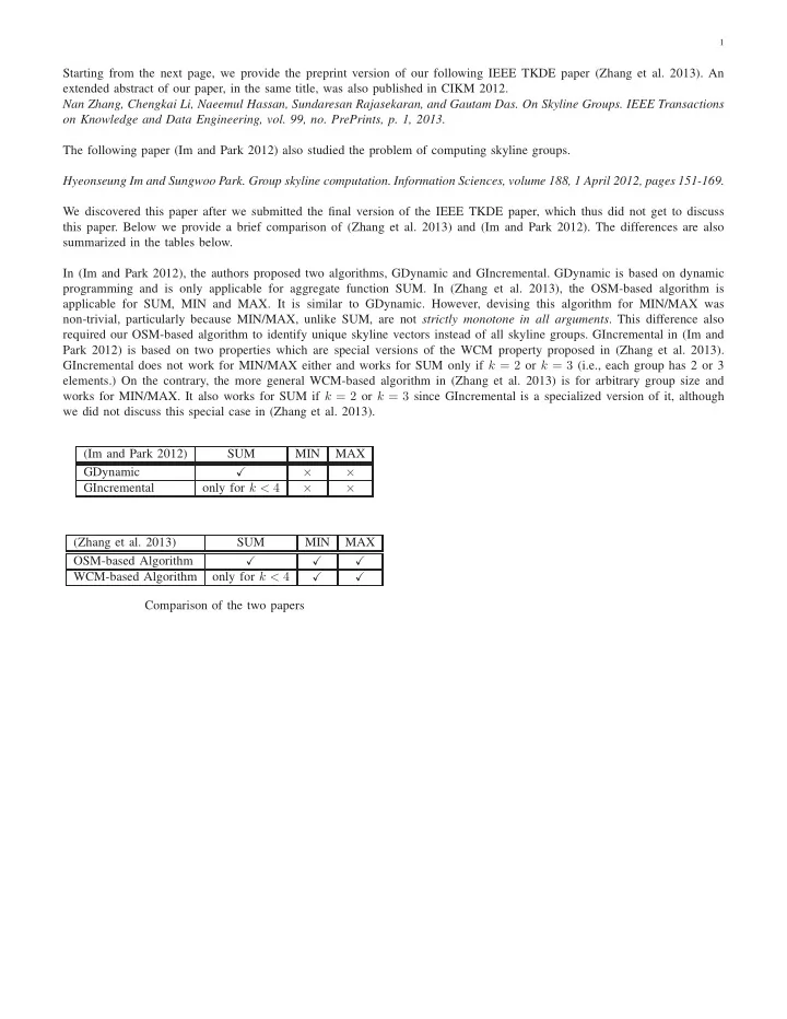
t1: -131,-40,-4,-4,-98,-20,4,4,-69,-49,-9,-49,-9,54,-59,16,20,20,-107,-22,27,-22,27,61,-39,13,17,13,17,68,-12,-12,89,59,82,35,29,29,46,51,40,51,40,55,27, 56,20,56,20,40,37,37,103,44,104,53,47,53,47,42,85,85,78,76,64,64,90,50,106 t2: -40,-79,-38,-38,-80,-66,-52,-52,-85,-59,-67,-59,-67,-54,14,-47,-15,-15,-56,0,-41,0,-41,1,-76,-18,-52,-18,-52,-22,-63,-63,18,-52,3,-50,-32,-32,-60,-11,- 47,-11,-47,-26,-67,-34,-51,-34,-51,-38,-59,-59,-22,-51,-18,-4,-32,-4,-32,-21,-17,-17,7,-27,-39,-39,-10,-39,-31 t3: -49,50,-28,-28,51,33,10,10,64,15,35,15,35,20,-102,39,-44,-44,39,-79,14,-79,14,-65,81,-22,28,-22,28,-13,58,58,-51,44,-63,15,-24,-24,62,-52,8,-52,8,- 31,57,-1,12,-1,12,-8,45,45,-7,19,6,-56,-8,-56,-8,-35,-9,-9,-68,-10,22,22,-30,5,25 t4: 15,-23,-34,-34,-9,-42,-49,-49,-15,-16,-39,-16,-39,-52,-24,-58,-55,-55,13,-27,-47,-27,-47,-57,-28,-46,-54,-46,-54,-71,-29,-29,-48,-59,-67,-60,-57,-57,- 41,-52,-55,-52,-55,-59,-53,-62,-54,-62,-54,-61,-50,-50,-68,-57,-75,-62,-63,-62,-63,-61,-63,-63,-63,-67,-64,-64,-72,-64,-70 t5: 67,39,75,-94,68,22,52,-62,58,145,57,-97,-32,-42,22,11,39,-84,86,94,82,-106,-107,-58,50,111,47,-144,-53,-50,130,-87,-77,-29,-42,-8,13,-54,8,51,28,- 129,-66,-41,7,39,20,-105,-33,-27,58,-75,-69,-22,-34,18,14,-95,-62,-32,51,-139,-61,-45,35,-89,-60,-27,-55 t6: 67,39,-94,75,68,22,-62,52,58,-97,-32,145,57,-42,22,11,-84,39,86,-106,-107,94,82,-58,50,-144,-53,111,47,-50,-87,130,-77,-29,-42,-8,-54,13,8,-129,- 66,51,28,-41,7,-105,-33,39,20,-27,-75,58,-69,-22,-34,-95,-62,18,14,-32,-139,51,-61,-45,-89,35,-60,-27,-55 t7:

94,-82,44,44,-25,-47,-3,-3,-83,12,-50,12,-50,-11,147,-90,56,56,-66,119,-40,119,-40,84,-122,46,-46,46,-46,20,-86,-86,90,-75,72,-40,30,30,-124,69,-

26,69,-26,38,-91,7,-22,7,-22,12,-71,-71,17,-34,-57,70,-5,70,-5,43,-13,-13,87,-5,-47,-47,38,-17,-54 t8: -28,93,75,75,21,95,95,95,68,46,101,46,101,123,-23,115,79,79,1,19,107,19,107,87,80,55,110,55,110,114,84,84,51,136,52,112,91,91,97,69,112,69,112, 101,109,96,104,96,104,104,111,111,111,119,104,73,107,73,107,93,100,100,77,119,114,114,101,115,130

TABLE 4: Counter-example for proving Theorem 3 Table 4. With this counter-example, {t1, t2, t3, t4} is a skyline group for SUM, whereas none of {t1, t2, t3}, {t1, t2, t4}, {t1, t3, t4}, or {t2, t3, t4} is on the 3-tuple skyline.

5 ALGORITHMS

5.1 Dynamic Programming Algorithm Based

Order-Specific Property Consider an arbitrary2 order of the n tuples in the input table, denoted by t1, . . . , tn. Let Tr be the set of the first r according to this order, i.e., Tr={t1, . . . , tr}. Let Skyr

be set of all skyline k-tuple groups with regard to Tr, i.e., each group in Skyr

k is not dominated by any other k-tuple

group consisting solely of tuples in Tr. One can see that

ur original problem can be considered as finding Skyn
k. We

now develop a dynamic programming algorithm which finds Skyn

k by recursively solving the “smaller” problems of finding

Skyn−1

and Skyn−1

k−1, etc.

For ease of presentation, we assume aggregate function SUM in all the propositions, algorithms, and explanations in this section. At the end of the section, we shall explain why the idea is also applicable for MIN and MAX. The algorithm is based on the following idea—All skyline k-tuple groups in Skyn

k can be partitioned into two disjoint sets S1 and S2

(Skyn

k ≡ S1 ∪ S2 and S1 ∩ S2 = ∅) according to whether

a group contains tn or not. In particular, S1 = {G|G ∈ Skyn

k, tn /

∈ G} and S2 = {G|G ∈ Skyn

k , tn ∈ G}. One can

see that S1 ⊆ Skyn−1

. On the other hand, S2 is subsumed by a set of groups that can be expanded from Skyn−1

k−1, the skyline

(k-1)-tuple groups with regard to Tn−1. More specifically, given a skyline k-tuple group that contains tn, if we remove tn from it, then the resulting group belongs to Skyn−1

k−1. These

two properties are formally presented as follows. proof. Note that Proposition 2 can be directly derived from Theorem 1. Proposition 1 Given G∈Skyn

k , if tn /

∈G, then G∈Skyn−1

. Proof: We prove this by contradiction. Assume G / ∈ Skyn−1

. Then, there must be a k-tuple group G′ ∈ Skyn−1

such that G′ ≻ G. There are two possible cases. (A) G′ ∈ Skyn

k: It contradicts with G ∈ Skyn k . (B) G′ /

∈ Skyn

k : There

must exist a k-tuple group G′′ ∈ Skyn

k such that G′′ ≻ G′.

2. We consider a random order in the experimental studies and leave the

problem of finding an optimal order (in terms of efficiency) to future work.

By transitivity of dominance relationship, G′′ ≻ G. This also contradicts with G ∈ Skyn

k. Hence G ∈ Skyn−1

. Proposition 2 Under aggregate function SUM, given G∈Skyn

k , if tn∈G, then G\{tn}∈ Skyn−1 k−1.

Algorithm 1: sky group(k, n): Dynamic programming algorithm based on order-specific property

Input: n: input tuples Tn={t1, . . . , tn}; k: group size; k ≤ n Output: Skyn

k : skyline k-tuple groups among Tn 1 if Skyn k is computed then 2

return Skyn

k ; 3 if k == 1 then 4

S+

2 ← {{tn}}; 5 else 6

S+

2 ← ∅; 7

Skyn−1

k−1 ← sky group(k-1, n-1); 8

foreach group G ∈ Skyn−1

k−1 do 9

candidate group ← G ∪ {tn};

S+

2 ← S+ 2 ∪ {candidate group}; 11 if k < n then 12

Skyn−1

(i.e., S+

1 ) ← sky group(k, n-1); 13 else 14

S+

1 ← ∅; 15 Cn k ← S+ 1 ∪ S+ 2 ; 16 Skyn k ← skyline(Cn k ); 17 return Skyn k ;

We further explain the dynamic programming algorithm by referring to the outline in Algorithm 1. The idea is also illustrated in Figure 2. The function sky group(k, n) is for finding Skyn

k. It first recursively computes Skyn−1

k−1 (Line

7). By adding tn into each group in Skyn−1

k−1 (Line 8-10),

the algorithm obtains a superset of the aforementioned S2, according to Proposition 2. We denote this superset S+

2 . By

recursively calling the sky group function (Line 12), it further computes Skyn−1

, which is a superset of the aforementioned S1, according to Proposition 1. We also denote Skyn−1

by S+

1 . S+ 1 and S+ 2 thus contain all necessary candidate groups

for Skyn

k. Thus, the skyline over candidate groups (Cn

k =S+ 1

∪ S+

2 , Line 15) is guaranteed to be equal to Skyn k . Existing

skyline query algorithms (e.g., [5], [10], [12]) can be applied

ver Cn

k . We use skyline() to refer to such algorithms (Line

16). The number of candidate groups considered (|S+

1 ∪ S+ 2 |)

can potentially be much smaller than the number of all possible

SLIDE 9

groups formed by all tuples, i.e., n

Note that Skyn

k is needed in calculating both Skyn+1 k

and Skyn+1

k+1. The algorithm recursively calls sky group(k, n)

inside sky group (k, n+1), to compute and memoize Skyn

Later it calls sky group(k, n) again inside sky group(k + 1, n+1). This time Skyn

k is not recomputed. Instead, the

stored result is directly used (Line 1). Hence it is a dynamic programming algorithm. The sequence of calculating Sky1

..., Skyn

k is shown by the dashed directed lines in Figure 2(b).

∪ ∪ ∪ ∪ add

1 1 − − n k

Sky

1 − n k

Sky

n k

Sky

k k

(a)

Sky

1 1 − − n k

Sky

1 − n

Sky

1 1 + −k n

Sky }} ,..., {{ ., . ,

1 k k k

t t e i Sky }} {{ ., . ,

1 1 1

t e i Sky

Sky

Sky }} ,..., {{ ., . ,

1 k k

t t e i Sky

(b)

Fig. 2: (a) Calculate Skyn

k from Skyn−1 k−1 and Skyn−1 k

; (b) Dynamic programming algorithm for calculating Skyn

Our discussion in this section so far assumed SUM. For MIN and MAX, Proposition 2 requires a small modification, as shown in the following Proposition 3. Proposition 3 Under aggregate function MIN and MAX, given G∈Skyn

k , if tn∈G, then there exists a group G′ ∈ Skyn−1 k−1

such that F(G′ ∪ {tn})=F(G). The implication of the applicability of Proposition 3 (instead

f Proposition 2) for MIN and MAX is that, if we still apply

Algorithm 1, the S+

2 produced by Line 8-10 is not guaranteed

to be a superset of the aforementioned S2. In other words, Line 16, which applies the skyline operation over candidate groups, cannot guarantee to produce Skyn

k. However, the algorithm

can still guarantee that the result of it contains all distinct aggregate vectors in Skyn

k, based on Proposition 3. Note

that our goal is to find all distinct skyline vectors and their accompanying (sample) skyline groups for MIN and MAX. Hence the algorithm suffices for our goal without change. 5.2 Iterative Algorithm Based on Weak Candidate-Generation Property The weak candidate-generation property (Definition 2) can be summarized as follows. Consider the scenario when every skyline group has a distinct aggregate vector. Given a skyline group G and any i, at least one i-tuple sub-group of G must be a skyline i-tuple group. Based on this property, Algorithm 2 iteratively generates candidate i-tuple groups by adding new tuples into skyline (i−1)-tuple groups (Line 6-12) and applies skyline algorithm over these candidates to find skyline i-tuple groups (Line 14). At every step of iteration, the algorithm

nly needs to generate i-tuple candidates by extending skyline

(i − 1)-tuple groups instead of all (i − 1)-tuple groups. Hence it effectively prunes candidate groups by generation. In reality, multiple skyline groups can have the same aggregate vector. The aforementioned statement is not true anymore. That is, given a skyline group G and any i, it is possible that none of its i-tuple sub-groups is a skyline i-tuple group. However, by Definition 2 and Theorem 2, a slightly different statement can be made for MIN and MAX—Given a skyline k-tuple group Gk and any i, there exists at least a skyline i- tuple group Gi that, when padded with other k−i tuples, will result in a skyline k-tuple group G′

k such that F(G′ k)=F(Gk).

Furthermore, given any skyline i-tuple group G′

i such that

F(G′

i)=F(Gi), we can pad G′ i with k−i other tuples to get

a skyline k-tuple group that has the same aggregate vector as Gk. Therefore, although Algorithm 2 does not produce all skyline groups, it guarantees to find all distinct skyline vectors. Algorithm 2: sky group(k, n): Iterative algorithm based

n weak candidate-generation property

Input: n: input tuples Tn={t1, . . . , tn}; k: group size; k ≤ n Output: Skyk: skyline k-tuple groups among Tn

1 C1 ← Tn; 2 Sky1 ← skyline(C1); 3 for i ← 2 to k do 4

//generate candidate i-tuple groups Ci from skyline i−1-tuple groups Skyi−1.

Ci ← ∅;

foreach G ∈ Skyi−1 do

foreach t ∈ Tn do

//generate candidate group

if t / ∈ G then

G′ ← G ∪ {t};

if G′ / ∈ Ci then

Ci ← Ci ∪ {G′};

//generate skyline i-tuple groups Skyi based on candidates Ci

Skyi ← skyline(Ci);

15 return Skyk

On Feasibility of Combining Order-Specific and Weak Candidate-Generation Properties: The order-specific and weak candidate-generation properties cannot be meaningfully

combined. The candidate and skyline groups generated in

Algorithm 2 are with respect to all n tuples, for different group size k. However, the candidate and skyline groups in Algorithm 1 are with respect to the first i (i=1..n) tuples by a particular order. The combination is possible at the last step of Algorithm 1. We can take the intersection of Cn

from Algorithm 1 and Ck from Algorithm 2 and then invoke skyline(Cn

k ∩ Ck). Even for this last step, the cost saving in

skyline() due to less candidates may not make up for the extra cost in producing both candidate sets Cn

k and Ck.

Complexity Analysis: The worst-case complexity of both Algorithms 1 and 2 is O( n

), which is as poor as the com-

plexity of the brute-force approach of enumerating all possible groups as candidates. We note that similarly the worst-case complexity of frequent itemset mining algorithms [1] is also exponential and equally poor as that of a brute-force approach. For both problems, it is the characteristics of real datasets that enables the algorithms to prune many candidates and thus to achieve better efficiency in reality. Specifically, one can see from Algorithms 1 and 2 that a critical factor determining the average-case complexity of these algorithms is the number

f unique i-tuple skyline vectors in a j-tuple subset of the

database (where i ∈ [1, k] and j ∈ [1, n]) - which in turn depends on the underlying data distribution. For example, the number of unique skyline vectors tends to be small when

SLIDE 10

values of different attributes are positively correlated: In the extreme-case scenario where all attributes share the same value, the number of unique skyline vector is always 1 for all i and j. On the other hand, there tends to be a large number of unique skyline vectors when the attributes are independently

distributed. We shall evaluate the efficiency of Algorithms 1

and 2 over real-world datasets in the experiments section. 5.3 From Distinct Vectors to Equivalent Groups For MIN and MAX, even the output size - i.e., the number

f skyline groups produced - may be too large to explicitly

compute and store. As discussed in Section 4.1, for output compression, we only need to retain one representative skyline group for each distinct aggregated vector. To be more specific, it is sufficient for Skyn

k in Algorithm 1 and Skyk

in Algorithm 2 to contain one representative group for each distinct aggregated vector of k-tuple groups. It can be easily achieved by a simple modification of the skyline algorithm at Line 16 of Algorithm 1 and Line 14 of Algorithm 2. Whenever a candidate group is compared with current groups in the skyline, we prune it if it is equivalent to some existing group. This will further reduce the size of candidate groups and the number of group comparisons in succeeding iterations. For input pruning, in the case of SUM and MIN, we remove all tuples dominated by at least k others. In the case of MAX, we remove all tuples not on the skyline. We showed in Section 4.2 that such input pruning techniques are safe - i.e., we will still obtain all distinct vectors and their representatives. As discussed in Section 4.1, although in many cases distinct vectors and their representative groups suffice, a user may request all skyline groups equivalent to a particular aggregated vector, for applying further criteria in choosing a group. To return such equivalent groups, various postprocessing steps are required, due to output compression and input pruning. Below we discuss such postprocessing for individual functions. Note that the same Algorithm 1 and 2 work if we do not apply output compression and input pruning. However, even if our application is to ultimately find all skyline groups, it is still beneficial to apply these two techniques and use postprocessing steps to find all skyline groups. Output compression and input pruning together not only reduce the output size, but also save computational cost by allowing the algorithms to deal with smaller input and intermediate results. In Section 6 we present experimental results to compare the execution time of

ur methods with and without k-dominator tuple pruning. The

results verify the benefit of applying this pruning technique regardless of the ultimate output—representative groups for all distinct aggregated vectors or all skyline groups. SUM: No postprocessing is necessary for SUM. First, a k- dominator tuple cannot appear in any skyline k-tuple group, as discussed in Section 4.2. Thus, input pruning will not trigger postprocessing for SUM. Second, if the ultimate goal is to fetch all skyline groups, output compression should not be applied, because there is no effective way of reconstructing skyline groups from distinct aggregated vectors. In Line 16

f Algorithm 1, all skyline i-tuple groups should be retained,

without applying the aforementioned simple modification that removes equivalent groups. Note that SUM only satisfies the

rder-specific property. Thus, only Algorithm 1 applies.

Algorithm 3: Finding skyline groups with identical aggregated vectors (MIN function)

Input: input tuples R; k: group size; k < |R| Output: Sky: skyline k-tuple groups for R

1 Sky ← ∅; 2 T ← remove k-dominator tuples from R; 3 n ← |T |; /* number the tuples in T as t1, ..., tn */ 4 Skyk ← sky group(k, n); /* Algorithm 1 or Algorithm 2 */ 5 foreach skyline k-tuple group G ∈ Skyk do 6

RG ← the set of tuples in R that dominate or are equivalent to the aggregated vector of G;

foreach k-combination G′ of tuples in RG do

Sky ← Sky ∪ {G′};

9 return Sky;

Algorithm 4: Finding skyline groups with identical aggregated vectors (MAX function)

Input: input tuples R; k: group size; k < |R| Output: Sky: skyline k-tuple groups among R

v ← the aggregated vector of G

candidate group ← ∅;

i ← 1;

p[1] ← null;

while i > 0 do

/* Note that it is fine to select a tuple multiple times because a tuple can get the same value as v on multiple dimensions. */

candidate group ← candidate group \ {p[i]};

p[i] ← get the next tuple in R that has v’s value on the ith dimension;

if p[i] == null then i ← i−1; continue;

candidate group ← candidate group ∪ {p[i]};

if |candidate group| > k then continue;

if i==d then

/* d is the number of dimensions. */ k′ ← k − |candidate group|;

if k′==0 then

Sky ← Sky ∪ {candidate group};

else

R′ ← R \ candidate group;

foreach k′-tuple combination G′ among the tuples in R′ do

Sky ← Sky ∪ {candidate group ∪ G′};

else

i ← i + 1;

p[i] ← null;

28 return Sky;

MIN: Two factors contribute to the need for postprocessing. First, the pruned k-dominator tuples may appear in skyline

groups. Second, the aforementioned equivalent group removal

performed at Line 16 of Algorithm 1 and Line 14 of Algo- rithm 2 will only keep one representative for each distinct aggregated vector. Note that both algorithms are applicable to MIN since MIN satisfies both order-specific and weak

SLIDE 11

candidate-generation properties. At the end of both algorithms, we obtain Skyk, which contains representatives of all distinct aggregated vectors, but not necessarily all skyline k-tuple

groups. To generate all skyline groups from Skyk for MIN, we

follow Algorithm 3. For each representative group, we find all the tuples that dominate or are equal to its aggregated vector. Any k−combination of these tuples is a skyline k-tuple group. This is based on the results from Section 4.1. MAX: Algorithms 1 and 2 are both applicable to MAX. Similar to MIN, MAX needs postprocessing due to both input pruning and output compression. We thus devise Algorithm 4 to produce all skyline groups from representative groups. For each representative group G that is found by Algo- rithms 1 and 2, Algorithm 4 uses a backtracking process to find all skyline groups that are equivalent to G. Denote the aggregated vector for G as v. On each dimension, we maintain a list of tuples from R (all input tuples to be considered) that attain v’s value on that dimension. We use the backtracking algorithm to enumerate all possible groups of the tuples from these lists, such that the groups have the same aggregated vector v and have less than or equal to k tuples. If a group has less than k tuples, it means there can be some “free” tuples. Any combination of other tuples will complement this group to form a skyline k-tuple group (Line 25-27). A special case for MAX function is when there is only one distinct aggregated vector, i.e., all skyline k-tuple groups reach the highest possible value on every dimension. In Algorithms 1 and 2, whenever an i-tuple candidate group (i ≤ k) is generated, we test if this group attains the highest possible value on every attribute. If so, we have already found the aggregated vector for all skyline groups. Using that vector, we either find one representative group or all skyline groups, by a backtracking process that is essentially the same as Algorithm 4. We omit the details.

6 EXPERIMENTS

The algorithms were implemented in C++. We executed all experiments on a Dell PowerEdge 2900 III server running Linux kernel 2.6.27-7, with dual quad-core Xeon 2.0GHz processors, 2x6MB cache, 8GB RAM, and three 250GB SATA HDs in RAID5. Datasets: We collected 512 tuples of NBA players who played in the 2009 regular season [20]. The tuple of each player has 5 statistics (i.e., 5 attributes) that measure the player’s performance. The statistics are points per game (PPG), rebounds per game (RPG), assists per game (APG), steals per game (SPG), and blocks per game (BPG). Players and groups of players are compared by these statistics and their aggregates. Another dataset is a collection of 35000 tuples that represent stocks for all the publicly traded firms as of December 31st, 2009 in several international markets [25]. Each tuple has 4 attributes, which are market capital (MC), stock price (SP), interest coverage ratio (ICR) and net income (NI). All the values were converted to US dollars. To study the scalability of our methods, we also experimented with synthetic datasets produced by the data generator in [5]. The datasets have 1 to 10 million tuples, on 5 attributes. The data generator allows us to produce datasets where the attributes are correlated, independent, and anti-correlated. In independent datasets, the attribute values of a tuple were generated by a uniform distribution. In correlated datasets, attribute values were generated using normal distributions. Anti-correlated datasets were generated by a more complex procedure, which involves adding and subtracting values from

therwise uniformly distributed attribute values.

Aggregate Functions and Methods Compared: We investigated the performance of the two algorithms discussed in Section 5, namely the algorithms based on order-specific property (OSM) and weak candidate-generation property (WCM). We also compared these methods with the baseline method (BASELINE), which is a direct adaptation of the general framework in [31] for our skyline group problem. (The detailed discussion of [31] is in Section 2.) We executed these methods for the aggregate functions discussed in previous sections—SUM, MIN, and MAX. Parameters: We ran our experiments under combinations of two parameter values, which are number of tuples, i.e., dataset size (n) and number of tuples per group, i.e., group size (k). Values Measured: For each applicable combination of aggregate function, method, and parameter values, we measured the execution time needed to find all distinct aggregate vectors and their representative groups, as well as the time to find all skyline groups. Besides execution time, we also measured the total number of candidate groups generated and number of pairwise group (aggregated vector) comparisons in the process. Due to the iterative nature of OSM and WCM, they call the basic skyline function multiple times. Hence, the total number of generated candidate groups is the cumulative sizes

f inputs to all skyline function invocations. Furthermore,

OSM produces candidate groups by merging two disjoint sets of smaller groups. Here input size was calculated as the summation of the sizes of disjoint sets.

n k = 2 k = 4 k = 6 G S V G S V G S V 1 M SUM 4×1011 247 247 4×1022 1654 1654 1×1033 6146 6146 MIN 187 141 1914 436 12816 870 MAX 368 220 147 73 2.9 M 1 4 M SUM 8×1012 219 219 1×1025 1610 1610 6×1036 7482 7482 MIN 179 131 2182 461 17784 1148 MAX 396 274 164 78 11 M 1 7 M SUM 2×1013 221 221 1×1026 1374 1374 2×1038 5825 5825 MIN 188 134 2193 455 16347 1002 MAX 552 323 354 90 55 M 1 10 M SUM 4×1013 210 210 4×1026 1300 1300 1×1039 4487 4487 MIN 183 133 2130 450 15442 913 MAX 402 224 968 63 0.8 B 1

TABLE 5: Number of all groups (G), skyline groups (S), distinct

skyline group vectors (V), under various n, k, and functions. Corre- lated synthetic dataset. M: million, B: billion

6.1 Study of Different Aggregate Functions Size of Output under Different Functions: Table 5 shows, for different n, k, and aggregate functions, the number of all possible groups (G), the number of all skyline groups (S), and the number of distinct aggregate vectors (V) for the skyline groups. The table is for correlated synthetic datasets. The observations made on the NBA dataset were similar. It can be seen that G quickly becomes very large, which

SLIDE 12

0.001 0.01 0.1 1 10 1 3 5 7 Execution Time Number of Tuples per Group 3 SUM 3 MAX 3 MIN

(a) n = 300

0.01 0.1 1 10 100 200 300 400 500 Execution Time Number of Tuples 3 SUM 3 MAX 3 MIN

(b) k = 3

10 100 1000 10000 100000 1e+06 1 3 5 7 Total Candidate Groups Number of Tuples per Group 3 SUM 3 MAX 3 MIN

1000 10000 100000 1e+06 100 200 300 400 500 Total Candidate Groups Number of Tuples 3 SUM 3 MAX 3 MIN

(d) k = 3

Fig. 3: (a)-(b): Execution time (seconds, log scale) and (c)-(d): number of candidate groups (log scale), mixture of SUM/MAX/MIN

PPG RBG APG SPG BPG G1 Carmelo Anthony Kobe Bryant Kevin Durant LeBron James Dwyane Wade 283.2 63.4 52.2 15.2 7.6 G2 Andrew Bogut Marcus Camby Monta Ellis Dwight Howard Josh Smith 166.2 96.4 32.2 13.4 19.4 G3 Trevor Ariza Monta Ellis Dwyane Wade Dwight Howard Josh Smith 202 72.6 43.2 16.6 14 G4 Carlos Boozer Baron Davis LeBron James Rajon Rondo Chris Paul 193.8 61.2 80.6 17.6 4.8 G5 Andrew Bogut LeBron James Chris Paul Dwight Howard Jason Kidd 185.8 81 64 14 13.8 PPG:Point Per Game, RBG: ReBound per Game, APG: Assist Per Game, SPG: Steal Per Game, BPG: Block Per Game

TABLE 6: Sample skyline groups from 512 players, 5 players per group indicates that any exhaustive method will suffer due to the large space of possible answers. We want to point out that the number of skyline vectors (V) can be large (e.g., under k=6). As discussed in Section 1, these distinct vectors become the input to further post-processing such as filtering, ranking and browsing. When a particular skyline vector is chosen by a user, the corresponding equivalent skyline groups are generated upon request. Among the three functions, in general SUM has the largest number of skyline vectors and MAX results in the smallest

utput size (V). This is due to the intrinsic characteristics
f these functions. In computing the aggregate vector for a

group, SUM reflects the strength of all group members on each

dimension. Hence it is more difficult for a group to dominate
r equal to another group on every dimension. In contrast,

MIN (MAX) chooses the lowest (highest) value among group members on each dimension. Hence skyline groups are formed by relatively small number of extremal tuples. On the other hand, if we compare the sizes of all skyline groups including the equivalent ones, it is rare under SUM to have multiple skyline groups sharing the same aggregate vec-

tor. MAX results in much more equivalent groups. Moreover,

under MAX, when group size k is larger than or equal to the number of attributes (5 for the datasets), all skyline groups have the same aggregate vector that attains the highest value

n every attribute.

Dealing with a Mixture of Aggregate Functions: Our methods allow a mixture of different aggregate functions applied on different attributes. OSM can handle arbitrary mixture

f SUM, MIN, and MAX, while WCM can handle any mixture
f MIN and MAX. Figure 3 shows the execution time of OSM
ver the 5-attribute NBA dataset, for 3 different mixtures of
functions. For example, 3SUM means SUM function on the

first 3 of the 5 attributes, and MIN and MAX on the remaining 2 attributes. From Figure 3 we can see that SUM function is typically more expensive. This is because output compression has less effect on SUM, under which it is more difficult for a group to dominate other groups. 6.2 Experiments on NBA Dataset Sample Resultant Skyline Groups: Table 6 shows several sample skyline 5-tuple groups under aggregate function SUM, from the NBA dataset. We see the sample groups are formed by elite players with different strengths. For instance, G1 is excellent in scoring (PPG), G2 excels in defense (RBG and BPG), and G3 is a very balanced group that is strong on many aspects although not the best on any dimension. Comparison of Various Methods: Figure 4-6 show the execution time and number of generated candidate groups, by BASELINE/OSM/WCM under all applicable functions, over the NBA dataset. Figure 7 further shows the number of pairwise group (aggregate vector) comparisons performed by these algorithms under MIN and MAX. In sub-figure (a) and (c) of these figures, we fix the size of dataset (n) to 300 tuples and vary group size (k). In sub-figure (b) and (d) of these figures, we fix the group size (k=5 for SUM/MIN and k=3 for MAX) and vary dataset size. We observed that OSM/WCM performed substantially (often orders of magnitude in execution time) better than BASELINE. Without the properties, BASELINE produced much more candidate groups than OSM/WCM and thus incurred much more pairwise group (aggregate vector) comparisons inside skyline function invocations. Effect of Input Pruning: Input pruning was applied in all the experiments for Figure 4-6. It had a good impact on the performance of all algorithms, since it significantly reduced the size of input. Table 7 shows that, in all considered cases on NBA dataset, less than 100 tuples remained after k-dominator tuple pruning was applied. Figure 8 shows that substantial saving on execution time was achieved for all functions.

n k = 1 k = 3 k = 5 k = 7 100 19 31 37 44 200 22 37 47 57 300 24 50 61 67 400 29 62 78 86 500 30 62 83 94

TABLE 7: Number of tuples dominated by < k tuples in NBA Search Space Pruning Power of OSM and WCM: Figure 5, 6 and 7 compare OSM and WCM, in terms of execution time, number of candidate groups produced, and number of pairwise group (aggregate vector) comparisons

incurred. We observed that, in terms of execution time, OSM

performed better than WCM on the NBA dataset under both MIN and MAX. Although WCM demonstrated better pruning power in most cases as it resulted in less candidate groups

SLIDE 13

0.001 0.01 0.1 1 10 100 1000 10000 1 3 5 7 Execution Time Number of Tuples per Group BASELINE OSM

(a) n = 300

1 10 100 1000 10000 100 200 300 400 500 Execution Time Number of Tuples BASELINE OSM

(b) k = 5

10 100 1000 10000 100000 1e+06 1e+07 1e+08 1e+09 1 3 5 7 Total Candidate Groups Number of Tuples per Group BASELINE OSM

10000 100000 1e+06 1e+07 1e+08 100 200 300 400 500 Total Candidate Groups Number of Tuples BASELINE OSM

(d) k = 5

Fig. 4: (a)-(b): Execution time (seconds, logarithmic scale) and (c)-(d): number of candidate groups (logarithmic scale), SUM

0.001 0.01 0.1 1 10 100 1000 10000 1 3 5 7 Execution Time Number of Tuples per Group BASELINE OSM WCM

(a) n = 300

0.1 1 10 100 1000 10000 100 200 300 400 500 Execution Time Number of Tuples BASELINE OSM WCM

(b) k = 5

10 100 1000 10000 100000 1e+06 1e+07 1e+08 1e+09 1 3 5 7 Total Candidate Groups Number of Tuples per Group BASELINE OSM WCM

1000 10000 100000 1e+06 1e+07 1e+08 100 200 300 400 500 Total Candidate Groups Number of Tuples BASELINE OSM WCM

(d) k = 5

Fig. 5: (a)-(b): Execution time (seconds, logarithmic scale) and (c)-(d): number of candidate groups (logarithmic scale), MIN

0.001 0.01 0.1 1 1 2 3 4 Execution Time Number of Tuples per Group BASELINE OSM WCM

(a) n = 300

0.001 0.01 0.1 100 200 300 400 500 Execution Time Number of Tuples BASELINE OSM WCM

(b) k = 3

10 100 1000 10000 100000 1 2 3 4 Total Candidate Groups Number of Tuples per Group BASELINE OSM WCM

100 1000 10000 100 200 300 400 500 Total Candidate Groups Number of Tuples BASELINE OSM WCM

(d) k = 3

Fig. 6: (a)-(b): Execution time (seconds, logarithmic scale) and (c)-(d): number of candidate groups (logarithmic scale), MAX

100 1000 10000 100000 1e+06 1e+07 1e+08 1e+09 1e+10 1 3 5 7 Total Comparisons Number of Tuples per Group BASELINE OSM WCM

(a) n = 300

10000 100000 1e+06 1e+07 1e+08 1e+09 1e+10 100 200 300 400 500 Total Comparisons Number of Tuples BASELINE OSM WCM

(b) k = 5

100 1000 10000 100000 1 2 3 4 Total Comparisons Number of Tuples per Group BASELINE OSM WCM

1000 10000 100000 100 200 300 400 500 Total Comparisons Number of Tuples BASELINE OSM WCM

(d) k = 3

Fig. 7: Number of pairwise group comparisons by different methods for MIN (a)-(b) and MAX (c)-(d)

0.1 1 10 100 200 300 400 500 Execution Time Number of Tuples With K-Dominator Pruning Without K-Dominator Pruning

(a) SUM

0.01 0.1 1 10 100 200 300 400 500 Execution Time Number of Tuples With K-Dominator Pruning Without K-Dominator Pruning

(b) MIN

0.01 0.1 1 100 200 300 400 500 Execution Time Number of Tuples With K-Dominator Pruning Without K-Dominator Pruning

Fig. 8: Effect of input pruning on OSM, k = 3

(Figures 5(c), 5(d), 6(c), and 6(d)), WCM required more pairwise group comparisons than OSM (Figure 7). Hence it lost in comparison with OSM. Effect of Output Compression: Figure 9 shows the cost (in execution time) of post-processing for obtaining all skyline groups from distinct skyline vectors, on the NBA dataset, for n = 100, MAX function, and OSM algorithm. We can see that in this configuration finding all skyline groups only doubled the execution time. This verifies that, even though the problem

f finding all skyline groups from distinct vectors is an NP-

hard problem, in practice it is usually efficient due to the small number of tuples that can “hit” MAX attribute values, as explained in Section 4.1. As n increases, naturally the cost

f post-processing will also increase. However, in reality we

may only need to produce the equivalent groups for a skyline vector chosen by the user, instead of for all skyline vectors.

0.005 0.01 0.015 0.02 1 2 3 4 Execution Time (second) Number of Tuples per Group Distinct Aggregated Vectors All Skyline Groups

Fig. 9: Finding all skyline groups for MAX, n= 100, OSM

6.3 Experiments on Stock Dataset We also experimented on the Stock dataset. As the behavior

f our algorithms on this dataset is mostly similar to that
n the NBA dataset, we do not present extensive results.

Figure 10 shows the performance of OSM and WCM for group size k = 3 under various input sizes. It is observed that, although the stock dataset is much bigger than the NBA dataset, the execution time is still considerably small. This is

SLIDE 14

1 2 3 4 5 6 7 10000 15000 20000 25000 30000 Execution Time Number of Tuples OSM

(a) SUM

0.2 0.25 0.3 0.35 0.4 0.45 0.5 0.55 0.6 0.65 0.7 0.75 10000 15000 20000 25000 30000 Execution Time Number of Tuples OSM WCM

(b) MIN

0.04 0.06 0.08 0.1 0.12 0.14 0.16 0.18 10000 15000 20000 25000 30000 Execution Time Number of Tuples OSM WCM

Fig. 10: Execution time (seconds, logarithmic scale) on stock dataset, k = 3

10 20 30 40 50 60 1 M 4 M 7 M 10 M Execution Time Number of Tuples OSM

(a) SUM

10 20 30 40 50 60 1 M 4 M 7 M 10 M Execution Time Number of Tuples OSM WCM

(b) MIN

5 10 15 20 1 M 4 M 7 M 10 M Execution Time Number of Tuples OSM WCM

Fig. 11: Execution time (seconds) of OSM/WCM on correlated synthetic dataset with 5 attributes, k = 4

10 100 1000 10000 2 3 4 5 Execution Time Number of Dimensions Anti-Correlated Independent Correlated

(a) SUM

10 100 2 3 4 5 Execution Time Number of Dimensions Anti-Correlated Independent Correlated

(b) MIN

1 10 100 2 3 4 5 Execution Time Number of Dimensions Anti-Correlated Independent Correlated

Fig. 12: Execution time (seconds, logarithmic scale) of OSM on different synthetic datasets, k = 3, n = 10 million

due to the effective input pruning. Table 8 shows that only less than 300 tuples remained after k-dominator tuple pruning was applied. We also see that, in this dataset, WCM took less execution time than OSM for MIN function. This is partly due to the overhead of OSM in performing candidate generation and skyline comparison for multiple (group size, table size) combinations, as mentioned in Section 4.3.1. 6.4 Experiments on Synthetic Datasets To show the scalability of our methods, we experimented on the synthetic datasets with 1 to 10 million tuples. In Figure 11, we see that OSM/WCM can finish within a minute on these large datasets, for k=4 and all 3 functions. The same methods will not be as efficient on independent

r even anti-correlated data. Figures 12 and

13 show the performance of OSM/WCM on three different datasets of equal cardinality, under different number of attributes. We see that the execution time on anti-correlated and independent data increases quickly and soon the algorithm cannot finish within reasonable amount of time. (Thus the corresponding bars are not plotted.) This is not surprising. In anti-correlated dataset, values of a tuple on different attributes are negatively

correlated. Hence it is more difficult to find a tuple dominating
ther tuples. This means input pruning in such a dataset cannot

reduce the input size effectively, and OSM/WCM cannot prune many candidates either. Attributes in real datasets may neither be fully correlated nor fully anti-correlated. The attributes

ften form groups, such as rebounds and blocks, assists

and steals in basketball games. The attributes within the same group are correlated, while the ones across different groups tend to be independent or anti-correlated. A direction for future

n k = 3 k = 5 k = 7 10000 99 139 178 15000 126 172 232 20000 130 180 239 25000 148 205 263 30000 143 217 281

TABLE 8: Number of tuples dominated by less than k tuples in

stock dataset

10 100 2 3 4 5 Execution Time Number of Dimensions Anti-Correlated Independent Correlated

(a) MIN

1 10 2 3 4 5 Execution Time Number of Dimensions Anti-Correlated Independent Correlated

(b) MAX

Fig. 13: Execution time (seconds, logarithmic scale) of WCM on

different synthetic datasets, k = 3, n = 10 million

study is to investigate the performance of our methods on synthetic data with such more realistic correlation patterns.

7 CONCLUSION

We proposed the novel problem of finding skyline groups which lends itself to many real-world applications. We developed novel algorithmic techniques on output compression, input pruning, and search space pruning to address the prob-

lem. For search space pruning, we identified a number of anti-

monotonic properties to efficiently remove non-skyline groups from consideration. Based on the properties, we developed dynamic programming and iterative algorithms for skyline group search. Experimental results on real and synthetic datasets verify that the proposed algorithms achieve orders of magnitude performance gain over the baseline method.

SLIDE 15

ACKNOWLEDGMENT

The work of Zhang is supported in part by NSF under grants 0852674, 0915834, and 1117297. The work of Li is partially supported by NSF grants 1018865, 1117369, and 2011, 2012 HP Labs Innovation Research Award. The work of Das is partially supported by NSF grants 0812601, 0915834, 1018865, a NHARP grant from the Texas Higher Education Coordinating Board, and grants from Microsoft Research and Nokia Research. Any opinions, findings, and conclusions or recommendations expressed in this publication are those of the author(s) and do not necessarily reflect the views of the funding agencies.

REFERENCES

[1]

R. Agrawal and R. Srikant. Fast algorithms for mining association rules

in large databases. In VLDB, 1994. [2]

A. Anagnostopoulos, L. Becchetti, C. Castillo, A. Gionis, and S. Leonar-
di. Power in unity: forming teams in large-scale community systems.

In CIKM, 2010. [3]

S. Antony, P. Wu, D. Agrawal, and A. El Abbadi. Moolap: Towards

multi-objective olap. In ICDE, 2008. [4] W.-T. Balke, U. Guntzer, and J. Zheng. Efficient distributed skylining for web information systems. In EDBT. 2004. [5]

S. B¨
rzs¨
nyi, D. Kossmann, and K. Stocker. The skyline operator. In

ICDE, 2001. [6]

C. Chan, H. Jagadish, K. Tan, A. Tung, and Z. Zhang.

Finding k- dominant skylines in high dimensional space. In SIGMOD, 2006. [7] C.-Y. Chan, H. Jagadish, K.-L. Tan, A. Tung, and Z. Zhang. On high dimensional skylines. In EDBT. 2006. [8]

S. Chaudhuri, N. Dalvi, and R. Kaushik. Robust cardinality and cost

estimation for skyline operator. In ICDE, 2006. [9] B.-C. Chen, K. LeFevre, and R. Ramakrishnan. Privacy skyline: privacy with multidimensional adversarial knowledge. In VLDB, 2007. [10] J. Chomicki, P. Godfrey, J. Gryz, and D. Liang. Skyline with presorting. In ICDE, 2003. [11] E. Dellis and B. Seeger. Efficient computation of reverse skyline queries. In VLDB, 2007. [12] P. Godfrey, R. Shipley, and J. Gryz. Maximal vector computation in large data sets. In VLDB, 2005. [13] H.T.Kung, F.Luccio, and F.P.Preparata. On finding the maxima of a set

f vectors. JACM, 22(4), 1975.

[14] D. Kossmann, F. Ramsak, and S. Rost. Shooting stars in the sky: an

nline algorithm for skyline queries. In VLDB, 2002.

[15] T. Lappas, K. Liu, and E. Terzi. Finding a team of experts in social

networks. In KDD, 2009.

[16] X. Lian and L. Chen. Monochromatic and bichromatic reverse skyline search over uncertain databases. In SIGMOD, 2008. [17] X. Lin, Y. Yuan, W. Wang, and H. Lu. Stabbing the sky: efficient skyline computation over sliding windows. In ICDE, 2005. [18] X. Lin, Y. Yuan, Q. Zhang, and Y. Zhang. Selecting stars: The k most representative skyline operator. In ICDE, 2007. [19] M. Morse, J. M. Patel, and H. V. Jagadish. Efficient skyline computation

ver low-cardinality domains. In VLDB, 2007.

[20] NBA Dataset. from http://www.databasebasketball.com/, 2012. [21] D. Papadias, Y. Tao, G. Fu, and B. Seeger. Progressive skyline computation in database systems. TODS, 2005. [22] J. Pei, B. Jiang, X. Lin, and Y. Yuan. Probabilistic skylines on uncertain

data. In VLDB, 2007.

[23] J. Pei, Y. Yuan, X. Lin, W. Jin, M. Ester, Q. Liu, W. Wang, Y. Tao,

J. X. Yu, and Q. Zhang. Towards multidimensional subspace skyline
analysis. TODS, 31(4), 2006.

[24] M. Sharifzadeh and C. Shahabi. The spatial skyline queries. In VLDB, 2006. [25] Stock Dataset. from http://pages.stern.nyu.edu/∼adamodar/New Home Page/data.html, 2012. [26] K.-L. Tan, P.-K. Eng, and B. C. Ooi. Efficient progressive skyline

computation. In VLDB, 2001.

[27] Y. Tao, L. Ding, X. Lin, and J. Pei. Distance-based representative

skyline. In ICDE, 2009.

[28] Y. Tao, X. Xiao, and J. Pei. Subsky: Efficient computation of skylines in subspaces. In ICDE, 2006. [29] P. Wu, C. Zhang, Y. Feng, B. Zhao, D. Agrawal, and A. El Abbadi. Parallelizing skyline queries for scalable distribution. In EDBT. 2006. [30] T. Xia and D. Zhang. Refreshing the sky: the compressed skycube with efficient support for frequent updates. In SIGMOD, 2006. [31] X. Zhang and J. Chomicki. Preference queries over sets. In ICDE, 2011. Nan Zhang received the BS degree in Computer Science from Peking University in 2001 and the PhD degree in Computer Science from Texas A&M University in 2006. He is an associate professor of Computer Science at the George Washington University. His current research interests include databases and information security/privacy. He is a member of the IEEE. Chengkai Li is an Assistant Professor in the Department of Computer Science and Engineer- ing at the University of Texas at Arlington. His research interests include databases, Web data management and data mining. In particular, he works on computational journalism, database exploration, database testing, entity search and query, and ranking and skyline queries. He received his Ph.D. degree in Computer Sci- ence from the University of Illinois at Urbana- Champaign in 2007, and an M.E. and a B.S. degree in Computer Science from Nanjing University, China, in 2000 and 1997, respectively. He is a member of the IEEE. Naeemul Hassan received his B.S. degree in Computer Science from Bangladesh University

f Engineering and Technology. He is currently a

Ph.D. candidate in the Department of Computer Science and Engineering at the University of Texas at Arlington. His research interests include skyline analysis, computational journalism, and social media analytics. Sundaresan Rajasekaran received an M.S. degree in Computer Science from the George Washington University and a B.E. degree in Computer Science from Anna University, India. He is currently a Ph.D. candidate in the De- partment of Computer Science at the George Washington University. His research interests include data privacy, network security and cloud computing. Gautam Das received the BTech degree in computer science from IIT Kanpur, India, and the PhD degree in computer science from the University of Wisconsin, Madison. He is a professor in the Computer Science and Engineering Department at the University of Texas, Arlington. Prior to joining the University of Texas, Arlington in Fall 2004, he held positions at Microsoft Re- search, Compaq Corporation, and the Univer- sity of Memphis. His research interests include data mining, information retrieval, databases, algorithms, and computational geometry. He is currently interested in ranking, top-k query processing, and sampling problems in databases as well as data management problems in the deep web, P2P and sensor networks, social networks, blogs, and web communities. His research has resulted in more than 130 papers which received several awards, including the IEEE ICDE 2012 Influential Paper award, VLDB journal special issue on best papers of VLDB 2007, best paper of ECML/PKDD 2006, and the best paper (runner up) of ACM SIGKDD

1998. He is on the editorial board of the journals the ACM Transactions
n Database Systems and the IEEE Transactions on Knowledge and

Data Engineering. He has served as the general chair of ICIT 2009, program chair of COMAD 2008, CIT 2004, and SIGMOD-DMKD 2004, and best paper awards chair of ACM SIGKDD 2006. His research has been supported by grants from US National Science Foundation, US Office of Naval Research, Department of Education, Texas Higher Education Coordinating Board, Microsoft Research, Nokia Research, Cadence Design Systems, and Apollo Data Technologies. He is a member of the IEEE.