Spatio-temporal Models Again point-referenced vs. areal unit data - PowerPoint PPT Presentation

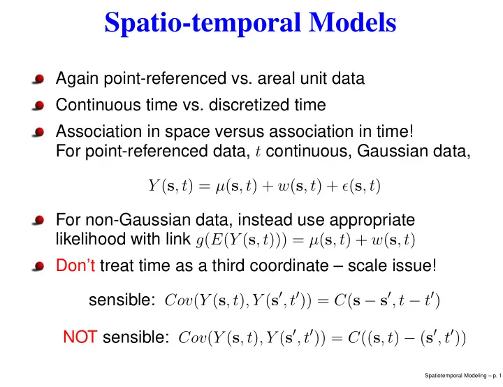
Spatio-temporal Models Again point-referenced vs. areal unit data Continuous time vs. discretized time Association in space versus association in time! For point-referenced data, t continuous, Gaussian data, Y ( s , t ) = µ ( s , t ) + w ( s , t ) + ǫ ( s , t ) For non-Gaussian data, instead use appropriate likelihood with link g ( E ( Y ( s , t ))) = µ ( s , t ) + w ( s , t ) Don’t treat time as a third coordinate – scale issue! sensible: Cov ( Y ( s , t ) , Y ( s ′ , t ′ )) = C ( s − s ′ , t − t ′ ) NOT sensible: Cov ( Y ( s , t ) , Y ( s ′ , t ′ )) = C (( s , t ) − ( s ′ , t ′ )) Spatiotemporal Modeling – p. 1

Spatio-temporal Models Separable form: C ( s − s ′ , t − t ′ ) = σ 2 ρ 1 ( s − s ′ ; φ 1 ) ρ 2 ( t − t ′ ; φ 2 ) Limitation Nonseparable form: Sum of independent separable processes More generally, mixing of separable covariance functions Spectral domain approaches - space-time spectral density and inverse Fourier transform Spatiotemporal Modeling – p. 2

Spatio-temporal Models An EDA idea Now suppose time is discretized, i.e. data are Y t ( s ) , t = 1 , . . . , T Type of data: time series versus cross-sectional (e.g., real estate sales). Latter is problematic For time series data, exploratory analysis: Arrange into an n × T matrix Y with entries Y t ( s i ) Center by row averages of Y yields Y rows Center by column averages of Y yields Y cols sample spatial covariance matrix: 1 T Y rows Y T rows sample autocorrelation matrix: 1 n Y T cols Y cols E , residuals matrix after a regression fitting Spatiotemporal Modeling – p. 3

Empirical Orthogonal Functions Can understand the structure of Y, Y rows , Y cols , E using empirical orthogonal functions Say for E , use singular value decomposition T E = UDV T = � d j u j v T j j =1 where U is n × n orthogonal, V is T × T orthogonal and D is “almost diagonal" If we arrange the d j in decreasing order then u j v T j is the j th empirical orthogonal function Typically, we only need a few terms in the sum to well approximate EE T . With just the first term it would suggest approximating E ( s , t ) by u 1 ( s ) v 1 ( t ) . Spatiotemporal Modeling – p. 4

Spatio-temporal Models If t discrete, a time series of spatial process realizations Modeling: Y t ( s ) = µ t ( s ) + w t ( s ) + ǫ t ( s ) , or perhaps g ( E ( Y t ( s )) = µ t ( s ) + w t ( s ) For ǫ t ( s ) , independent N (0 , τ 2 t ) For w t ( s ) w t ( s ) = α t + w ( s ) , α t ∼ ? w t ( s ) independent for each t w t ( s ) = w t − 1 ( s ) + η t ( s ) , independent spatial process innovations Inference? Interpolate for new locations at an observed time; predict for a current location at a new time; new location and new time Spatiotemporal Modeling – p. 5

Multivariate spatio-temporal models Again, connecting space and time, extending versions above Y ( s, t ) = µ ( s, t ) + w ( s, t ) + ǫ ( s, t ) with µ ( s, t ) = X ( s, t ) T β For w ( s, t ) , can supply an additive form in random effects Can supply a multiplicative form in random effects (from EOF idea) Perhaps, most natural is a coregionalization specification Spatiotemporal Modeling – p. 6

cont. Coregionalization approach In the LMC, consider w ( s, t ) = A v ( s, t ) where the components of v ( s , t ) are independent univariate space-time processes Can extend to A t , to A ( s ) or even A ( s, t ) Can make the evolution dynamic, e.g., w t ( s ) = A v t ( s ) where v lt ( s ) = φv l,t − 1 ( s ) + ǫ lt ( s ) Further variations Could also try cross-convolution using valid C l ( s, t ) Spatiotemporal Modeling – p. 7

Dynamic Space Time models Again, t is discrete. More general two-stage specification. Dynamics in the mean Stage 1: Measurement equation Y ( s, t ) = µ ( s, t ) + ǫ ( s, t ) ; ǫ ( s, t ) ind 0 , σ 2 � � ∼ N . ǫ µ ( s, t ) = x T ( s, t ) ˜ β ( s, t ) . ˜ β ( s, t ) = β t + β ( s, t ) Stage 2: Transition equation ind � � β t = β t − 1 + η t , η t 0 , Σ η ∼ N p . β ( s, t ) = β ( s, t − 1) + w ( s, t ) . w ( s, t ) is a multivariate space-time process Spatiotemporal Modeling – p. 8

cont. So, as above w ( s, t ) = A v ( s, t ) , with v ( s, t ) = ( v 1 ( s, t ) , ..., v p ( s, t )) T . The v l ( s, t ) are replications of a Gaussian processes with unit variance and correlation function ρ l ( φ l , · ) Can connect to linear Kalman filter Spatiotemporal Modeling – p. 9

An example: Modelling Temperature given precipitation. Sampled temperature data (maximum monthly temperature) and sampled precipitation data (maximum monthly precipitation), 50 sites across Colorado, January through December in 1997 (12 months). temp ( s, t ) = ˜ β 0 ( s, t ) + ˜ β 1 ( s, t ) precip ( s, t ) + ǫ ( s, t ) Independent Gaussians for η t Space-time varying intercept process and slope process. Coregionalization for w ( s, t ) Spatiotemporal Modeling – p. 10

Spatial domain (with elevation) 41 41 40 40 Latitude 39 39 38 38 37 37 −108 −108 −106 −106 −104 −104 −102 −102 Longitude Spatiotemporal Modeling – p. 11

Parameter estimates Parameters median (2.5%, 97.5%) Σ η [1 , 1] 0.296 (0.130, 0.621) Σ η [2 , 2] 0.786 (0.198, 1.952) � Σ η [1 , 2] Σ η [1 , 1] Σ η [2 , 2] -0.562 (-0.807, -0.137) Σ w [1 , 1] 0.017 (0.016, 0.019) Σ w [2 , 2] 0.026 (0.0065, 0.108) � Σ w [1 , 2] Σ w [1 , 1] Σ w [2 , 2] -0.704 (-0.843, -0.545) σ 2 0.134 (0.106, 0.185) ǫ 1.09 (0.58, 2.04) φ 1 φ 2 0.58 (0.37, 1.97) Range for intercept process 2.75 (1.47, 5.17) Range for slope process 4.68 (1.60, 6.21) Spatiotemporal Modeling – p. 12

Time varying parameters Intercept beta_0t 1.5 1.5 1.5 0.0 0.0 0.0 Jan Mar May Jul Sep Nov Month Coeff. of Precipitation −0.5 −0.5 −0.5 beta_1t −2.0 −2.0 −2.0 Jan Mar May Jul Sep Nov Month Spatiotemporal Modeling – p. 13

Intercept process Time-sliced image-contour plots displaying the posterior mean surface of the spatial residuals Jan Feb Mar Apr 41 41 41 41 41 41 41 41 40 40 40 40 40 40 40 40 Latitude Latitude Latitude Latitude 39 39 39 39 39 39 39 39 38 38 38 38 38 38 38 38 37 37 37 37 37 37 37 37 −108 −108 −104 −104 −108 −108 −104 −104 −108 −108 −104 −104 −108 −108 −104 −104 Longitude Longitude Longitude Longitude May Jun Jul Aug 41 41 41 41 41 41 41 41 40 40 40 40 40 40 40 40 Latitude Latitude Latitude Latitude 39 39 39 39 39 39 39 39 38 38 38 38 38 38 38 38 37 37 37 37 37 37 37 37 −108 −108 −104 −104 −108 −108 −104 −104 −108 −108 −104 −104 −108 −108 −104 −104 Longitude Longitude Longitude Longitude Sep Oct Nov Dec 41 41 41 41 41 41 41 41 40 40 40 40 40 40 40 40 Latitude Latitude Latitude Latitude 39 39 39 39 39 39 39 39 38 38 38 38 38 38 38 38 37 37 37 37 37 37 37 37 −108 −108 −104 −104 −108 −108 −104 −104 −108 −108 −104 −104 −108 −108 −104 −104 Spatiotemporal Modeling – p. 14 Longitude Longitude Longitude Longitude

Slope process Time-sliced image-contour plots displaying the posterior mean surface of the spatial residuals Jan Feb Mar Apr 41 41 41 41 41 41 41 41 40 40 40 40 40 40 40 40 Latitude Latitude Latitude Latitude 39 39 39 39 39 39 39 39 38 38 38 38 38 38 38 38 37 37 37 37 37 37 37 37 −108 −108 −104 −104 −108 −108 −104 −104 −108 −108 −104 −104 −108 −108 −104 −104 Longitude Longitude Longitude Longitude May Jun Jul Aug 41 41 41 41 41 41 41 41 40 40 40 40 40 40 40 40 Latitude Latitude Latitude Latitude 39 39 39 39 39 39 39 39 38 38 38 38 38 38 38 38 37 37 37 37 37 37 37 37 −108 −108 −104 −104 −108 −108 −104 −104 −108 −108 −104 −104 −108 −108 −104 −104 Longitude Longitude Longitude Longitude Sep Oct Nov Dec 41 41 41 41 41 41 41 41 40 40 40 40 40 40 40 40 Latitude Latitude Latitude Latitude 39 39 39 39 39 39 39 39 38 38 38 38 38 38 38 38 37 37 37 37 37 37 37 37 −108 −108 −104 −104 −108 −108 −104 −104 −108 −108 −104 −104 −108 −108 −104 −104 Spatiotemporal Modeling – p. 15 Longitude Longitude Longitude Longitude

Multivariate Dynamic Model For ( s , t ) yielding Y ( s , t ) = ( Y 1 ( s , t ) , ..., Y p ( s , t )) T , and covariate vectors (including an intercept) x l ( s, t ) , l = 1 , 2 , ..., p . The model becomes Y ( s, t ) = µ ( s, t ) + ǫ ( s, t ) ; ǫ ( s, t ) ind ∼ N ( 0 , Σ ǫ ) ; Σ ǫ = σ 2 ǫ I p µ ( s, t ) = X ( s, t ) ˜ β ( s, t ) , � T � T T is � m where ˜ ˜ 1 ( s, t ) , ..., ˜ β ( s, t ) = m ( s, t ) l =1 k l × 1 , β β is p × � m � x T 1 ( s, t ) , ..., x T � X ( s, t ) = Diag m ( s, t ) l =1 k l . Spatiotemporal Modeling – p. 16