Spatio-temporal correlations across the melting of 2 D Wigner - - PowerPoint PPT Presentation

Spatio-temporal correlations across the melting of 2D Wigner molecules

Amit Ghosal IISER KOLKATA

• Coulomb interacting particles in 2D confinements.
• Static & Dynamic responses across ‘melting’.
• Effect of ‘Disorder/irregularity’ on melting.

Computational Tools

• Molecular dynamics and Classical (Metropolis) Monte

Carlo with Simulated Annealing at finite T.

• Path integral Quantum Monte Carlo (QMC) at low T; variational and

diffusion QMC at T = 0.

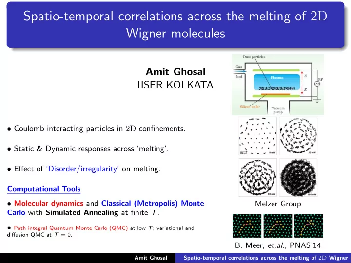
Melzer Group

• B. Meer, et.al., PNAS’14

Amit Ghosal Spatio-temporal correlations across the melting of 2D Wigner m

Crystal of Coulomb particles and its melting:

Wigner Crystal Melting (1934) Competetion between PE & KE

Coulomb repulsion forces particles to stay as far as possible from each other, localizing them in a crystal. Kinetic Energy delocalizes them. KE ∼ kBT (equipartition) ⇒ Thermal / Classical melting [Gann, Chakravarty & Chester, 1979] KE ∼ Quantum (zero-point) fluctuations ⇒ Quantum melting. [Tanatar & Ceperley, 1989]

• In confinements, Wigner Crystal ⇒ “Wigner Molecule”

H = q2 4πǫ

N

• i<j

1 | ri − rj | +

N

• i

Vconf (ri ); r = | r| =

• x2 + y 2

(a) Irregular: V Ir

conf(r) = a{x4/b+by4−2λx2y2+γ(x−y)xyr}

(b) Circular: V Cr

conf(r) = αr2, with α = mω2/2 Amit Ghosal Spatio-temporal correlations across the melting of 2D Wigner m

Thermal melting of Wigner Molecules (WM)

T=0.002 T=0.015 T=0.065 (a)T=0 (b)T=0.0150 (b)T=0.0650

Amit Ghosal Spatio-temporal correlations across the melting of 2D Wigner m

Static Correlations: EPJB 86, 499, (2013), arXiv:1701.02338

Lindemann:

L =

1 N

N

i=1 a−1 i

• |

ri − r 0

i |2

1 2 3 4 5 0.02 0.04 0.06 0.08 0.1

T LR

N=50 N=75 N=101 N=141

Specific Heat: cV = d ˆ

E dT = T −2

E2 − E2

0.02 0.04 0.06 0.08 0.1 T cV 50 100 150 0.02 0.03 0.04 0.05 N Tc N=145 N=121 N=76 N=56 Γ

c = 137

BOO: ψ6(i) = N

k=1 1 Nb

Nb

l=1 ei6θki

2 4 6 8 10 12 0.2 0.4 0.6 0.8 1

(a) VIr

Conf

N=500 P(|ψ6|) |ψ6|

T=0.002 T=0.006 T=0.010 T=0.020 T=0.030 T=0.050 0.2 0.4 0.6 0.8 1

(b) VCr

Conf

N=500 |ψ6|

1 2 3 4 5 0.2 0.4 0.6 0.8 1 (c) VIr

Conf

N=500 P(φ6) φ6 T=0.002 T=0.006 T=0.010 T=0.020 T=0.030 T=0.050 0.2 0.4 0.6 0.8 1 (d) VCr

Conf

N=500 φ6

m6(i): projection of ψ6(i) onto mean local orientation field. m6(i) =

• ψ∗

6 (i) 1 Nb

Nb

k=1 ψ6(k)

• Larsen & Grier, PRL ’96
• Also studied g(r), g6(r), Generalized susceptibilities: χψ, χφ

Amit Ghosal Spatio-temporal correlations across the melting of 2D Wigner m

Take-home messages from static correlations & questions:

• 1. Crossover from ‘solid’-like to ‘liquid’-like behavior discerned from

independent observables (unique Tx within tolerance).

• 2. No apparent distinction between TX (within errorbars) in circular and

irregular confinements.

• 3. Qualitative responses are more-or-less independent of N (for

100 ≥ N ≤ 100) though there are differences in details. What can dynamics tell us about the ‘solid’ and ‘liquid’ in traps? Can motional signatures distinguish the crossover based on the nature of the confinement? (e.g., circular vs. irregular) Can we access generic signatures of disordered dynamics in traps?

EPL, 114, 46001 (2016); arXiv:1701.02338; and unpublished

Amit Ghosal Spatio-temporal correlations across the melting of 2D Wigner m

Displacements [∆ r (t) = { r (t) − r (0)}] in ‘solid’

• Spatially correlated inhomogeneous motion at large t even at low T in irregular traps.

y

T = 0.006 t = 100

(a)VIr

Conf

r/r0 ≤ 0.15 0.15<r/r0 ≤ 0.50

T = 0.006 t = 1000

(b) VIr

Conf

0.50<r/r0≤1.0

T = 0.006 t = 9500

(C)VIr

Conf

r/r0>1.0

y x

T=0.006 t=100

(d) VCr

Conf

x

T=0.006 t=1000

(e) VCr

Conf

x

T=0.006 t=9500

(f) VCr

Conf

Amit Ghosal Spatio-temporal correlations across the melting of 2D Wigner m

spatio-temporal density correlations:

Dynamical (spatio-temporal) information best extracted from Van-Hove correlation function: G(r, t) = N

i,j=1 δ

• r − |

ri(t) − rj(0)|

• Self-part Gs(r, t) (when i = j): probability to move on an average a distance r in time t.

10-4 10-2 100 0.5 1 2 2.5 Irregular (T=0.006) Gs(r,t) r/r0 t= 1 10 100 1000 9500 10-4 10-2 100 0.5 1 2 Gs(r,t) r/r0 t = 200 400 700 1000

10-4 10-2 100 4 8 15

Irregular (T=0.030) Gs(r,t) r/r0 1 10 100 200 400 1000 9500 10-4 10-2 100 0.5 1 2 2.5 Circular (T=0.006) Gs(r,t) r/r0

10-4 10-2 100

1 2

Gs(r,t) r/r0 t = 200 400 700 1000

10-4 10-2 100 4 8 15

Circular (T=0.030) Gs(r,t) r/r0 t = 1 10 100 200 400 1000 9500

Amit Ghosal Spatio-temporal correlations across the melting of 2D Wigner m

Stretched exponential decay of spatial correlation in IWM

Observation:

• Gs(r, t) ∼ e−r2/c for small r ∀t.
• Gs(r, t) shows complex tail (large t).

Postulate: G small

s

(r, t) ∼ e−r2/c for r ≤ rc and G large

s

(r, t) ∼ e−lrk for r > rc

• Optimal rc and other parameters (including k) determined by minimizing total χ2.

0.4 0.6 1.0 2.0 10-1 100 101 102 (a) VIr

Conf

k t

0.3 1.0 2.0 10-1 100 101 102 103 104 k

t

T=0.020 T=0.030 T=0.050

100 101 102 (b) VCr

Conf

t T=0.002 T=0.006 T=0.020 T=0.030

0.3 1.0 2.0 10-1 100 101 102 103 104

k t

T=0.075 T=0.100 T=0.250

• Small t, All T: k ≃ 2, (Gaussian tail).
• Large t, Low T: (IWM + CWM) k ∼ 1 (exponential tail)

[P. Chaudhuri et al., PRL (2007)]

• Large t, High T: • (CWM) 1 ≥ k ≤ 2, (stretched Gaussian tail); Expt: [He et al. ACS Nano (’13)]
• (IWM) k < 1, T-dependent Stretched exponential tail of spatial correlation!

Amit Ghosal Spatio-temporal correlations across the melting of 2D Wigner m

Time scales: α− relaxation time from overlap Function

0.2 0.4 0.6 0.8 1 10-1 100 101 102 103 104 (a) VIr

Conf

Q(t) t

0.2 0.4 0.6 0.8 1 100 101 102 103 104 (b) VCr

Conf

Q(t) t

T=0.002 T=0.006 T=0.010 T=0.020 T=0.030 T=0.050 100 101 102 0 0.015 0.03 0.045

τα T

100 101 102 0 0.015 0.03 0.045

τα T 0.2 0.4 0.6 0.8 100 101 102 103 104

(a) VIr

Conf

Χ4(t)

t

T=0.002 T=0.006 T=0.010 T=0.020 T=0.030 T=0.050

0.3 0.6 0.9 1.2 100 101 102 103 104 (b) VCr

Conf

Χ4(t)

t

100 101 0.02 0.04

τx T

100 101

0.02 0.04

τx T

• 2

2 30 90 150

log τα 1/T

N=75 N=150 N=500

• 2

2 30 90 150

log τα 1/T

• Q(t) = 1

N

N

• i=1

W (| ri(t) − ri(0)|) where W (ri) = 1 if ri < rcut, & W (ri) = 0 if ri > rcut (satisfied once,

• nly on first passage).

[Kob et al. (’12); Karmakar et al. (’14)]

• α− relaxation time (τα) from Q(t):

Q(τα) = e−1

• χ4(t) = 1

N [Q2(t) − Q(t)2]

[Karmakar et.al. PNAS, (’08)]

• χ4(t) measures extent of dynamic heterogeneity (spatial correlations in particles’ dynamics).
• τx(T) is the time-scale when dynamic heterogeneity is maximum at the given T.

Amit Ghosal Spatio-temporal correlations across the melting of 2D Wigner m

Dynamical Correlations

0.1 0.2 0.4 0.6 0.8 1 10-1 100 101 102 103 104 (a) VIr

Conf N=150

Cg(t) t

T=0.002 T=0.006 T=0.010 T=0.020 T=0.030 T=0.050 100 101 102 103 104 (b) VCr

Conf N=150

t

• When particles’ cages rearrange, the

system relaxes & particles diffuse. ⇒ corresponding structural change characterized by a cage correlation (CC) function. Cage correlation function: Cg(t) = L(i)(t)·L(i)(0)

L(i)2(0) [Rabani et.al. PRL’99]

• Cg(t) ∼ exp[−(t/τg)c]; c ∼ 0.5 for

irregular, and c ∼ 0.6 for circular traps.

• Persistence time (τp, solid line): a

particle displaced beyond a cut-off for the first time.

• Exchange time (τe, dotted line):

time required for subsequent passage by cut-off distance. [Hedges et. al., J. Chem.

Phys.(2007)]

• Two distributions decouple for

Irregular confinement but signature of decoupling is weaker for Circular confinement.

0.1 0.2 0.3 0.4 0.5 0.6

• 1

1 2 3 4 5 6 7 (a) VIr

Conf

N =500 P(log(τ)) log(τ) τp, T=0.020 τe, T=0.020 T=0.030 T=0.050 T=0.100

• 1

1 2 3 4 5 6 7 (b) VCr

Conf

N=500 log(τ)

Amit Ghosal Spatio-temporal correlations across the melting of 2D Wigner m

Quantum Melting in confinements

• Hamiltonian (for Harmonic trap):

H =

N

• i=1
• − n2

2 ∇2

i + r2 i

• +

N

• i<j

1 rij n = √ 2l2

0 /r2 0 , l2 0 = /mω0

(E0 = e2/ǫr0 = mω2

0/2) and rs = 1/n2.

n = 0 ⇒ classical, increase of n induces quantum fluctuations. Included: Zero-point motion / quantum dynamics. Quantum statistics: Boltzmannons (PIMC), Spin- 1

2 Fermions (VMC + DMC)

Thermal fluctuations → tortuous path of melting. Quantum fluctuations →diffusion around equilibrium position. A study similar to that on bulk systems.

• B. Clark, M. Casula, and D. Ceperley PRL (2009)

[D. Bhattacharya et.al. EPJ.B, 89, 60 (2016)]

n=0.01

T=0.005 n=0.06

n=0.10

n=0.15

T=0.010

T=0.020 T

T=0.030

n

Amit Ghosal Spatio-temporal correlations across the melting of 2D Wigner m

Acknowledging Collaborators

Students: (IISER K) Biswarup Ash Dyuti Bhattacharya Anurag Banerjee Collaborators: Jaydeb Chakrabarti (SNBNCBS Kolkata) Chandan Dasgupta (IISc Bangalore)

Also:

• A. V. Fillinov & M. Bonitz (Kiel U. Germany)

Amit Ghosal Spatio-temporal correlations across the melting of 2D Wigner m

Conclusions

1 Spatio-temporal correlations chracterize ‘solid’ to ‘liquid’ crossover in

Wigner molecules.

2 TX is not sensitive to N or confinement geometry for 100 ≤ N ≤ 500. 3 Intriguing motional signatures for confined Coulomb particles! 4 Multiple time-scales for relaxation identified.

• Complex motion yields slow relaxations, akin to supercooled liquids.

5

Outlook:

• ”Glassiness” and the role of defects?
• Classical vs. Quantum dynamics, observables?

Amit Ghosal Spatio-temporal correlations across the melting of 2D Wigner m