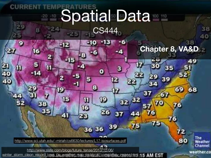
Spatial Data CS444 Chapter 8, VA&D - - PowerPoint PPT Presentation

Spatial Data

CS444

http://www.slate.com/blogs/future_tense/2013/12/06/ winter_storm_cleon_record_lows_us_weather_map_today_is_completely_insane.html http://www.sci.utah.edu/~miriah/cs6630/lectures/L17-isosurfaces.pdf

Chapter 8, VA&D

Recap

• So far, we’ve studied methods to determine the

position of a data point on the screen

• graph drawing, treemaps, scatterplots, PCA
• However, some datasets come with very good

positional information

• Wind maps, weather simulations, CT scans

How do we represent spatial data?

• In the real world, there’s

infinitely many data points in a weather map

• In a computer, we only have

finite memory and finite time

• How do we solve this

problem?

Finite-dimensional function spaces

• Some functions can be represented succinctly

2

• 2

1 1 f(x) = ⇢ 1, if − 1

2 ≤ x ≤ 1 2

0,

• therwise

Finite-dimensional function spaces

• Some functions can be represented succinctly

2

• 2

1 1

f(x) =    1 + x, if − 1 ≤ x ≤ 0 1 − x, if 0 ≤ x ≤ 1 0,

• therwise

Finite-dimensional function spaces

• Build complicated functions by sums of shifted,

scaled versions of these simple functions

Finite-dimensional function spaces

• Build complicated functions by sums of shifted,

scaled versions of these simple functions 2

• 2

1 1

• 1

Finite-dimensional function spaces

2

• 2

1 1

• 1
• Build complicated functions by sums of shifted,

scaled versions of these simple functions

Finite-dimensional function spaces

2

• 2

1 1

• 1
• Build complicated functions by sums of shifted,

scaled versions of these simple functions

Finite-dimensional function spaces

2

• 2

1 1

• 1
• Build complicated functions by sums of shifted,

scaled versions of these simple functions

Finite-dimensional function spaces

2

• 2

1 1

• 1
• Build complicated functions by sums of shifted,

scaled versions of these simple functions

Finite-dimensional function spaces

2

• 2

1 1

• 1
• Build complicated functions by sums of shifted,

scaled versions of these simple functions

Finite-dimensional function spaces

2

• 2

1 1

• 1
• Build complicated functions by sums of shifted,

scaled versions of these simple functions

Finite-dimensional function spaces

2

• 2

1 1

• 1
• Build complicated functions by sums of shifted,

scaled versions of these simple functions

2

• 2

1 1

• 1

f(x) = X

i

ϕ(x − i)ci

ϕ(x)

2

• 2

1 1

• 1

f(x) = X

i

ϕ(x − i)ci

sums shifts scales

simple functions

ϕ(x)

Example: nearest-neighbor interpolation

2

• 2

1 1 ϕ(x)

Example: linear interpolation

ϕ(x) 2

• 2

1 1

• 1

Alternative formulation: f(x) = v0(1 − x) + v1x

Cubic Interpolation

ϕ(x)

Cubic Interpolation

ϕ(x) Alternative formulation:

What is “Correct” Interpolation?

What is “Correct” Interpolation?

ϕ(x)

Cubic, (etc) Approximation

http://www.cs.berkeley.edu/~sequin/CS284/IMGS/ makingbasisfunctions.gif

Why go through this trouble?

• Why not just define these functions “procedurally”?
• At the end of the day they’re just arrays and if

statements, after all

• Because we can do math on those sums more

easily

Derivatives of finite- dimensional function spaces

f(x) = X

i

ciϕ(x − i) d f dx(x) = d dx X

i

ciϕ(x − i)

Derivatives of finite- dimensional function spaces

f(x) = X

i

ciϕ(x − i)

d f dx(x) = X

i

d dxciϕ(x − i)

Derivatives of finite- dimensional function spaces

d f dx(x) = X

i

ci dϕ dx (x − i)

f(x) = X

i

ciϕ(x − i)

• Derivatives are just another type of function

space where all we do is change the “simple function”

Derivatives of finite- dimensional function spaces

d f dx(x) = X

i

ci dϕ dx (x − i)

f(x) = X

i

ciϕ(x − i)

Derivatives of finite- dimensional function spaces

ϕ(x) dϕ dx (x)

Multidimensional functions

ϕ(x) Basis function for bilinear interpolation

f(x, y) = v00 (1 − x) (1 − y) + v10 (x) (1 − y) + v01 (1 − x) (y) + v11 (x) (y)

Interlude: The Gradient of a Function

rf(~ x) =  @f/@x @f/@y

• But what is that?

Interlude: The Gradient of a Function

First we remember our friend the Taylor series: Now we ask ourselves: if we move a little away from , in what direction does grow the fastest? f (x0, y0) f ✓ x y ◆ = f ✓ x0 y0 ◆ + rf ✓ x0 y0 ◆T  x x0 y y0

• + ε

Interlude: The Gradient of a Function

f ✓ x y ◆ = f ✓ x0 y0 ◆ + rf ✓ x0 y0 ◆T  x x0 y y0

• + ε

rf ✓ x0 y0 ◆T  dx dy

• =

 ∂f/∂x ∂f/∂y T  dx dy

Interlude: The Gradient of a Function

max  ∂f/∂x ∂f/∂y T  dx dy

•  ∂f/∂x

∂f/∂y

•  dx

dy

Interlude: The Gradient of a Function

max  ∂f/∂x ∂f/∂y T  dx dy

•  ∂f/∂x

∂f/∂y

•  dx

dy

• 

dx dy

• = rf

|rf|

Interlude: The Gradient of a Function

max  ∂f/∂x ∂f/∂y T  dx dy

• 

dx dy

• = rf

|rf|

The gradient points in the direction of greatest increase and its length is the rate of greatest increase

Visualizing Scalar Fields

Colormapping

• “Default” strategy:
• create color scale using

the range of the function as the domain

• f the scale
• create a position scale

to convert from the domain of the function to positions on the screen

• set the pixel color

according to the scale

Colormapping guidelines apply!

Applies to “abstract” spaces too

http://www.nytimes.com/interactive/2015/04/16/upshot/ marriage-penalty-couples-income.html?abt=0002&abg=0

Contouring: isolines

Contouring: isolines

http://ryanhill1.blogspot.com/2011/07/isoline-map.html

Contouring: isolines

How do we compute them?

Contouring: isolines

http://ryanhill1.blogspot.com/2011/07/isoline-map.html

Approach to Contouring in 2D

• Contour must cross every grid line connecting two

grid points of opposite sign

530 - Introduction to Scientific Visualization Oct 7, 2014,

Interpolate along grid lines

+

• x

x

Get cell Identify grid lines w/cross Find crossings Primitives naturally chain together

Cases

No Crossings Case Polarity Rotation Total x2 2 Singlet x2 8 x4 Double adjacent x2 4 x2 (4) Double Opposite x2 2 x1 (2) (x2 for polarity) 16 = 24

+

Ambiguities

• How to form lines?
• How to form the lines?

x x x x

Ambiguities

• Right or Wrong?
• Right or wrong?

x x x x x x x x x x x x

Contouring: isolines