Sound Waves Our aim is to model the propagation of sound. Until - - PowerPoint PPT Presentation

Sound Waves

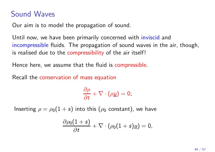
Our aim is to model the propagation of sound. Until now, we have been primarily concerned with inviscid and incompressible fluids. The propagation of sound waves in the air, though, is realised due to the compressibility of the air itself! Hence here, we assume that the fluid is compressible. Recall the conservation of mass equation ∂ρ ∂t + ∇ · (ρu) = 0; Inserting ρ = ρ0(1 + s) into this (ρ0 constant), we have ∂ρ0(1 + s) ∂t + ∇ · (ρ0(1 + s)u) = 0,

49 / 57

Sound Waves

• r

ρ0 ∂s ∂t + ∇(ρ0(1 + s)) · u + ρ0(1 + s)∇ · u = 0, giving ∂s ∂t + ∇s · u + (1 + s)∇ · u = 0. The terms ∇s · u and s∇ · u are small considering s and u are small, hence we can neglect them to obtain ∂s ∂t + ∇ · u = 0.

50 / 57

Sound Waves

Recall the momentum equations ∂u ∂t + (u · ∇)u = −∇p ρ + g. We assume no external forces, and hence g = 0. The flow is slow and slowly varying, hence we assume (u · ∇)u = 0. Thus the momentum equation becomes ∂u ∂t = −∇p ρ

• r

ρ∂u ∂t = −∇p.

51 / 57

Sound Waves

We also assume that p is a function of ρ only. Thus, Taylor’s theorem yields p(ρ) = p(ρ0 + ρ0s) = p(ρ0) + ρ0sp′(ρ0) + ... As s is small, we can truncate after the second term the Taylor expansion, to get p(ρ) = p(ρ0 + ρ0s) = p(ρ0) + ρ0sp′(ρ0). Inserting this into the momentum equations, we obtain ρ0(1 + s)∂u ∂t = −∇(p(ρ0 + ρ0s)) = −∇(p(ρ0) + ρ0sp′(ρ0)) = −p′(ρ0)ρ0∇s.

52 / 57

Sound Waves

Assuming that s ∂u

∂t is small, we neglect it also, and we obtain

∂u ∂t + c2∇s = 0, where c2 = p′(ρ0). Differentiating ∂s

∂t + ∇ · u = 0 with respect to time, we obtain

0 = ∂2s ∂t2 + ∂ ∂t ∇ · u = ∂2s ∂t2 + ∇ · ( ∂ ∂t u). Making use of ∂u

∂t + c2∇s = 0, on the second term on the right-hand side

• f the previous relation, we conclude

0 = ∂2s ∂t2 + ∇ · (−c2∇s)

• r

∂2s ∂t2 = c2∆s.

53 / 57

Wave Equation

The equation ∂2s ∂t2 = c2∆s is known as the wave equation. Remark: The wave equation, together with Laplace’s equation and the heat equation they constitute the 3 fundamental examples of the classical theory of (second order) partial differential equations. BIG IDEA: The wave equation models simple travelling waves. Note: The wave equation does not model any dissipation, i.e., the waves that models do not decay as they approach infinity...

54 / 57

Wave Equation

The constant c in ∂2s ∂t2 = c2∆s is known as the wave speed. Example: Consider the wave equation in 1 space dimension; i.e., ∂2s ∂t2 = c2 ∂2s ∂x2 . If s is of the form s(t, x) = A sin(kx) sin(ωt), we obtain from the wave equation ω2 = c2k2. Hence, s(t, x) = A sin(kx) sin(ωt) is a solution of the wave equation iff ω = ck. ω is called frequency and k is the amplitude of the wave in this case.

55 / 57