Some very cool things about Sage Or, why I am excited about Sage - - PowerPoint PPT Presentation

Some very cool things about Sage

Or, why I am excited about Sage Franco V. Saliola saliola@gmail.com

Laboratoire de Combinatoire et d’Informatique Math´ ematique Universit´ e du Qu´ ebec ` a Montr´ eal

LaCIM Seminar 7 March 2008

Sage is a distribution of open-source software.

Sage is a distribution of open-source software.

Software included with Sage : ATLAS

Automatically Tuned Linear Algebra Software

BLAS

Basic Fortan 77 linear algebra routines

Bzip2

High-quality data compressor

Cddlib

Double Description Method of Motzkin

Common Lisp

Multi-paradigm and general-purpose programming lang.

CVXOPT

Convex optimization, linear programming, least squares

Cython

C-Extensions for Python

F2c

Converts Fortran 77 to C code

Flint

Fast Library for Number Theory

FpLLL

Euclidian lattice reduction

FreeType

A Free, High-Quality, and Portable Font Engine

Sage is a distribution of open-source software.

Software included with Sage : G95

Open source Fortran 95 compiler

GAP

Groups, Algorithms, Programming

GD

Dynamic graphics generation tool

Genus2reduction

Curve data computation

Gfan

Gr¨

• bner fans and tropical varieties

Givaro

C++ library for arithmetic and algebra

GMP

GNU Multiple Precision Arithmetic Library

GMP-ECM

Elliptic Curve Method for Integer Factorization

GNU TLS

Secure networking

GSL

Gnu Scientific Library

JsMath

JavaScript implementation of LaTeX

Sage is a distribution of open-source software.

Software included with Sage : IML

Integer Matrix Library

IPython

Interactive Python shell

LAPACK

Fortan 77 linear algebra library

Lcalc

L-functions calculator

Libgcrypt

General purpose cryptographic library

Libgpg-error

Common error values for GnuPG components

Linbox

C++ linear algebra library

Matplotlib

Python plotting library

Maxima

computer algebra system

Mercurial

Revision control system

MoinMoin

Wiki

Sage is a distribution of open-source software.

Software included with Sage : MPFI

Multiple Precision Floating-point Interval library

MPFR

C library for multiple-precision floating-point computations

ECLib

Cremona’s Programs for Elliptic curves

NetworkX

Graph theory

NTL

Number theory C++ library

Numpy

Numerical linear algebra

OpenCDK

Open Crypto Development Kit

PALP

A Package for Analyzing Lattice Polytopes

PARI/GP

Number theory calculator

Pexpect

Pseudo-tty control for Python

PNG

Bitmap image support

Sage is a distribution of open-source software.

Software included with Sage : PolyBoRi

Polynomials Over Boolean Rings

PyCrypto

Python Cryptography Toolkit

Python

Interpreted language

Qd

Quad-double/Double-double Computation Package

R

Statistical Computing

Readline

Line-editing

Rpy

Python interface to R

Scipy

Python library for scientific computation

Singular

fast commutative and noncommutative algebra

Scons

Software construction tool

SQLite

Relation database

Sage is a distribution of open-source software.

Software included with Sage : Sympow

L-function calculator

Symmetrica

Representation theory

Sympy

Python library for symbolic computation

Tachyon

lightweight 3d ray tracer

Termcap

for writing portable text mode applications

Twisted

Python networking library

Weave

Tools for including C/C++ code within Python

Zlib

Data compression library

ZODB

Object-oriented database

Sage is a distribution of open-source software.

Software included with Sage : Sympow

L-function calculator

Symmetrica

Representation theory

Sympy

Python library for symbolic computation

Tachyon

lightweight 3d ray tracer

Termcap

for writing portable text mode applications

Twisted

Python networking library

Weave

Tools for including C/C++ code within Python

Zlib

Data compression library

ZODB

Object-oriented database

Plus additional optional packages

Sage is a distribution of mathematics software.

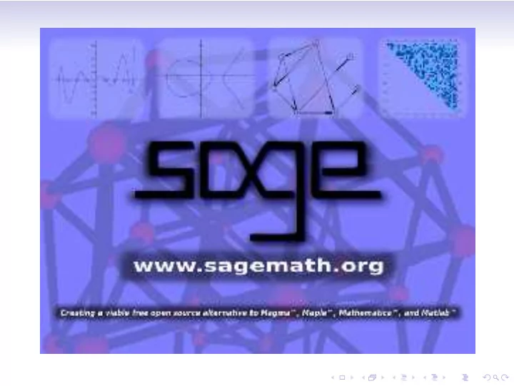
Sage’s mission: “Creating a viable, free, open-source alternative to MagmaTM, MapleTM, MathematicaTM, and MatlabTM.”

Sage is a distribution of mathematics software.

Sage’s mission: “Creating a viable, free, open-source alternative to MagmaTM, MapleTM, MathematicaTM, and MatlabTM.” Algebra GAP, Maxima, Singular Algebraic Geometry Singular, Macaulay2 Arbitrary Precision Arithmetic GMP, MPFR, MPFI, NTL, . . . Arithmetic Geometry PARI, NTL, mwrank, ecm, . . . Calculus Maxima, Sympy Combinatorics Symmetrica, MuPAD-Combinat∗ Exact Linear Algebra Linbox, IML Graph Theory NetworkX Graphics MatPlotLib, Tachyon3d Group theory GAP Numerical Linear Algebra GSL, Scipy, Numpy

Sage is a distribution of free, open-source software.

“You can read Sylow’s Theorem and its proof in Huppert’s book in the library . . . then you can use Sylow’s Theorem for the rest of your life free of charge, but for many computer algebra systems license fees have to be paid regularly . . . .

Sage is a distribution of free, open-source software.

“You can read Sylow’s Theorem and its proof in Huppert’s book in the library . . . then you can use Sylow’s Theorem for the rest of your life free of charge, but for many computer algebra systems license fees have to be paid regularly . . . . With this situation two of the most basic rules of conduct in mathematics are violated: In mathematics information is passed on free of charge and everything is laid open for checking.”

Sage is a distribution of free, open-source software.

“You can read Sylow’s Theorem and its proof in Huppert’s book in the library . . . then you can use Sylow’s Theorem for the rest of your life free of charge, but for many computer algebra systems license fees have to be paid regularly . . . . With this situation two of the most basic rules of conduct in mathematics are violated: In mathematics information is passed on free of charge and everything is laid open for checking.” — J. Neub¨ user (1993) (started GAP in 1986)

Sage is a distribution of free, open-source software.

You have the freedom: to run the program, for any purpose. to study how the program works, and adapt it to your needs. to redistribute copies so you can help your neighbour. to improve the program, and release your improvements to the public, so that the whole community benefits.

Sage is a distribution of free, open-source software.

You have the freedom: to run the program, for any purpose. to study how the program works, and adapt it to your needs. to redistribute copies so you can help your neighbour. to improve the program, and release your improvements to the public, so that the whole community benefits. Also, you don’t have to pay for it.

The Sage programming language is Python

Python is a powerful, modern, interpreted programming-language.

The Sage programming language is Python

Python is a powerful, modern, interpreted programming-language. Interpreted means it works like Maple or Mathematica. python: x = 17 python: x 17 python: x**2 289

The Sage programming language is Python

Python is a powerful, modern, interpreted programming-language. Interpreted means it works like Maple or Mathematica. python: x = 17 python: x 17 python: x**2 289 It’s easy to learn. Lots of free documentation. http://diveintopython.org/ http://docs.python.org/tut/

The Sage programming language is Python

The Sage programming language is Python

It’s easy to read and write.

• 17x
• x ∈ {0, 1, . . . , 9} and x is odd
• python: [17*x for x in range(0,10) if x%2 == 1]

The Sage programming language is Python

It’s easy to read and write.

• 17x
• x ∈ {0, 1, . . . , 9} and x is odd
• python: [17*x for x in range(0,10) if x%2 == 1]

Lots of Python libraries: databases, graphics, networking, . . .

The Sage programming language is Python

It’s easy to read and write.

• 17x
• x ∈ {0, 1, . . . , 9} and x is odd
• python: [17*x for x in range(0,10) if x%2 == 1]

Lots of Python libraries: databases, graphics, networking, . . . It is easy to use C/C++ libraries from within Python.

The Sage programming language is Python

It’s easy to read and write.

• 17x
• x ∈ {0, 1, . . . , 9} and x is odd
• python: [17*x for x in range(0,10) if x%2 == 1]

Lots of Python libraries: databases, graphics, networking, . . . It is easy to use C/C++ libraries from within Python. Cython: Python code − → compiled C code.

The Sage programming language is Python

“Google has made no secret of the fact they use Python a lot for a number of internal projects. Even knowing that, once I was an employee, I was amazed at how much Python code there actually is in the Google source code system.” — Guido van Rossum (creator of Python)

Several ways to use Sage

A library for Python scripts. #!/usr/bin/env sage -python import sys from sage.all import *

Several ways to use Sage

Command line interface.

• | SAGE Version 2.10.1, Release Date: 2008-02-02

| | Type notebook() for the GUI, and license() for information. |

• sage: 17^2

289 sage: |

Several ways to use Sage

Graphical notebook: online at sagenb.org

Sage plays well with L

AT

EX

L

AT

EX input: \begin{sagesilent} var(’s t’) f = t^2*e^t-sin(t) \end{sagesilent} Let $f(t)=\sage{f}$. Then the Laplace tranform

• f $f$ is: $\sage{f.laplace(t,s)}$.

Sage plays well with L

AT

EX

L

AT

EX input: \begin{sagesilent} var(’s t’) f = t^2*e^t-sin(t) \end{sagesilent} Let $f(t)=\sage{f}$. Then the Laplace tranform

• f $f$ is: $\sage{f.laplace(t,s)}$.

L

AT

EX output: Let f(t) = t2et − sin (t) . Then the Laplace tranform of f is:

2 (s−1)3 − 1 s2+1.

Sage plays well with L

AT

EX

L

AT

EX input: Here is an example of a tree: \sageplot{Graph({0:[1,2,3], 2:[5]}).plot()}

Sage plays well with L

AT

EX

L

AT

EX input: Here is an example of a tree: \sageplot{Graph({0:[1,2,3], 2:[5]}).plot()} L

AT

EX output: Here is an example of a tree:

Sage plays well with L

AT

EX

L

AT

EX input: \sageplot{plot(-x^3+3*x^2+7*x-4,-5,5)}

Sage plays well with L

AT

EX

L

AT

EX input: \sageplot{plot(-x^3+3*x^2+7*x-4,-5,5)} L

AT

EX output:

Sage plays well with L

AT

EX

L

AT

EX input:

\begin{sagesilent} t6 = Tachyon(camera_center=(0,-4,1), xres = 800, yres = 600, \ raydepth = 12, aspectratio=.75, antialiasing = True) t6.light((0.02,0.012,0.001), 0.01, (1,0,0)) t6.light((0,0,10), 0.01, (0,0,1)) t6.texture(’s’, color = (.8,1,1), opacity = .9, specular = .95, \ diffuse = .3, ambient = 0.05) t6.texture(’p’, color = (0,0,1), opacity = 1, specular = .2) t6.sphere((-1,-.57735,-0.7071),1,’s’) t6.sphere((1,-.57735,-0.7071),1,’s’) t6.sphere((0,1.15465,-0.7071),1,’s’) t6.sphere((0,0,0.9259),1,’s’) t6.plane((0,0,-1.9259),(0,0,1),’p’) \end{sagesilent} \sageplot{t6}

Sage plays well with L

AT

EX

L

AT

EX output:

The Sage community

Many people have contributed to Sage (directly & indirectly). There are several mailing lists. http://www.sagemath.org IRC: #sage-devel on freenode.org. Developers are very friendly and helpful.

Let’s use Sage

Let’s use Sage

Demo 0: Get help. Start typing, then hit TAB. CommandName? for documentation and examples. CommandName?? for docs, examples and source code.

Let’s use Sage

Demo 1: Interfaces. sage: %maple

• -> Switching to Maple <--

maple: f := x -> x^2 f := proc (x) options operator, arrow; x^2 end proc maple: D(f)(x) 2*x maple: exit

• -> Exiting back to SAGE <--

sage:

Let’s use Sage

Demo 1: Interfaces. sage: %gap

• -> Switching to Gap <--

gap: s8 := Group( (1,2), (1,2,3,4,5,6,7,8) ) Group([ (1,2), (1,2,3,4,5,6,7,8) ]) gap: a8 := DerivedSubgroup( s8 ) Group([ (1,2,3), (2,3,4), (2,4)(3,5), (2,6,4), (2,4)(5,7), gap: Size( a8 ); IsAbelian( a8 ); IsPerfect( a8 ) 20160 false true

Let’s use Sage

Demo 2: String manipulation Let P0 = {} and Pn = PowerSet(Pn−1). Examples:

P1 = {{}} P2 = {{{}} , {}} P3 = {{{{}} , {}} , {} , {{}} , {{{}}}}

We want the words obtained from the elements in Pn by replacing each { with a and each } with b. Examples:

P1 → [ab] . P2 → [ab, aabb] . P3 → [ab, aabb, aaabbb, aaabbabb] .

Let’s use Sage

# Import a module (library) import string # Define a function to generate the sets def P(n): if n == 0: return Set([]) else: return Subsets(P(n-1)) # Define a function to the replacing. f = lambda x : str(x).translate(string.maketrans(’{}’,’ab’),’, ’) # Do a list comprehension to combine them. words = lambda n : [f(x) for x in P(n)]

Let’s use Sage

Demo 3: Sloane sage: seqs = sloane_find([1,1,2,3,5,8,13],1) sage: for x in seqs: ....: print x[1] Fibonacci numbers: F(n) = F(n-1) + F(n-2), F(0) = 0, F(1) = 1, F(2) = 1, ...

Let’s use Sage

Demo 4: Play with Partitions Set of Partitons

P = Partitions(6) P.list() P.count() P.<tab>

individual partitons

nu = Partitions(6).random(); nu nu = Partition([3,2,2,1]) print nu.ferrers_diagram() nu.hook_lengths() nu.conjugate() nu.hook_product(x) nu.hook_product(1) nu.<tab>

Let’s use Sage

Demo 5: Play with Symmetric Functions

Help: SymmetricFunctionAlgebra? Power basis: p = SymmetricFunctionAlgebra(QQ, basis=’power’); p Expand: p([3]).expand(4) Elementary basis: e = SFAElementary(QQ) Monomial basis: m = SFAMonomial(QQ) Homogeneous basis: h = SFAHomogeneous(QQ) Schur basis: s = SFASchur(QQ) Dual basis: m.dual_basis() is h Omega: m([2,2,1]).omega() Change of basis: m(h([3])) Change of basis matrix: h.transition_matrix(m,4) Plethysm: s([3])(s([3,2]))

Let’s use Sage++

Demo 6: Play with Jack and Macdonald Polynomials sage: H = MacdonaldPolynomialsH(QQ); H sage: s = SFASchur(H.base_ring()); s sage: s(H([2])) sage: _.expand(3) sage: J = JackPolynomialsJ(QQ,t=1); J sage: s = SFASchur(J.base_ring()); s sage: nu = Partitions(7).random(); nu sage: J(nu) sage: s(J([3,2,2,1])) sage: nu.hook_product(1)

Let’s use Sage++

Demo 7: Manipulate sage: @manipulate sage: def _(a=(0,1)): ....: x,y = var(’x,y’) ....: show(plot3d(sin(x*cos(y*a)), \ ....: (x,0,5), (y,0,5)), figsize=4)

Let’s use Sage++

Demo 8: Posets sage: P = Poset([[1,2],[4],[3],[4],[]]); P sage: P.antichains() sage: P.show() sage: P.is_meet_semilattice() sage: P.is_graded() sage: Pi = PosetOfIntegerPartitions(5); Pi sage: Pi.show() sage: B = BooleanLattice(5); B sage: B.show() sage: PosetOfRestrictedIntegerPartitions(7).show()

Let’s use Sage

Demo 9: Rubik’s cube sage: C = RubiksCube().scramble() sage: C.show() sage: C.show3d() sage: C.solve()

Let’s use Sage

Demo 10: Linear Algebra & Sudoku Solver sage: A = matrix(ZZ,9,[5,0,0, 0,8,0, 0,4,9, \ 0,0,0, 5,0,0, 0,3,0, \ 0,6,7, 3,0,0, 0,0,1, \ 1,5,0, 0,0,0, 0,0,0, \ 0,0,0, 2,0,8, 0,0,0, \ 0,0,0, 0,0,0, 0,1,8, \ 7,0,0, 0,0,4, 1,5,0, \ 0,3,0, 0,0,2, 0,0,0, \ 4,9,0, 0,5,0, 0,0,3]); A sage: A.determinant() sage: A.minpoly() sage: sudoku(A)