Some Special Cases Recall: we can classify models: constant - - PowerPoint PPT Presentation

Some Special Cases

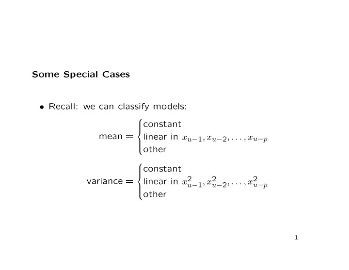
• Recall: we can classify models:

mean =

      

constant linear in xu−1, xu−2, . . . , xu−p

• ther

variance =

      

constant linear in x2

u−1, x2 u−2, . . . , x2 u−p

• ther

1

Autoregressions

• The simplest special case is the autoregression.
• If:

µt = linear function of xt−1, xt−2, . . . , xt−p = φ1xt−1 + φ2xt−2 + · · · + φpxt−p and σ2

t = constant

= τ2 then Xt is called autoregressive of order p (AR(p)).

2

• We usually define

ǫt = Xt − E

Xt| Xt−1, Xt−2, . . .

• = Xt −
• φ1Xt−1 + φ2Xt−2 + · · · + φpXt−p
• .
• We then write the model as

Xt = φ1Xt−1 + φ2Xt−2 + · · · + φpXt−p + ǫt where E

ǫt| Xt−1, Xt−2, . . . = 0,

and Var

ǫt| Xt−1, Xt−2, . . . = τ2.

3

• If in addition the shape of the conditional density is fixed,

then the ǫ’s are independent and identically distributed.

• The polynomial

φ(z) = 1 −

• φ1z + φ2x2 + · · · + φpzp

, where we view z as a complex variable, plays an important role in the theory of autoregressions.

4

• In particular, if the zeros of φ(z) are outside the unit circle,

then: – 1/φ(z) has a Taylor series expansion 1 φ(z) = 1 + ψ1z + ψ2z2 + . . . which converges for |z| ≤ 1; – Xt is a linear combination of ǫt, ǫt−1, . . . : Xt = ǫt + ψ1ǫt−1 + ψ2ǫt−2 + . . .

5

• These equations are often written in terms of the back-shift
• perator B, defined by

BXt = Xt−1, Bǫt = ǫt−1, . . .

• Then

ǫt = Xt −

• φ1Xt−1 + φ2Xt−2 + · · · + φpXt−p
• = Xt −
• φ1BXt + φ2B2Xt + · · · + φpBpXt
• = φ(B)Xt.

6

• So it is natural to write

Xt = 1 φ(B)ǫt =

• 1 + ψ1B + ψ2B2 + . . .
• ǫt

= ǫt + ψ1ǫt−1 + ψ2ǫt−2 + . . .

7

Conditional Heteroscedasticity: ARCH

• Another special case is Engle’s AutoRegressive Conditionally

Heteroscedastic, or ARCH, model.

• If

µt = constant and σ2

t = linear function of x2 t−1, x2 t−2, . . . , x2 t−q

= ω + α1x2

t−1 + α2x2 t−2 + · · · + αqx2 t−q

then Xt is called AutoRegressive Conditionally Heteroscedas- tic of order q (ARCH(q)).

8

• ARCH models are important in finance, because many finan-

cial time series show variances that fluctuate over time, while usually having constant, essential zero, conditional means.

−0.20 −0.10 0.00 0.10 diff(log(spx$Close)) 1950 1960 1970 1980 1990 2000 2010

Logarithmic returns on the S&P500 Index 9

A Modest Generalization

• In practice, large values of p or q are sometimes needed to

get a good fit with the AR(p) and ARCH(q) models.

• That introduces many parameters to be estimated, which is

problematic.

• We need models that allow large p with few parameters.

10

• Suppose for instance that

Xt = θXt−1 − θ2Xt−2 − · · · + ǫt for some θ, −1 < θ < 1.

• That is, p = ∞, but φr = −(−θ)r ⇒ only one parameter, θ.
• Then

ǫt = Xt − θXt−1 + θ2Xt−2 + · · · = 1 1 + θBXt,

• r

Xt = (1 + θB)ǫt = ǫt + θǫt−1.

11

• This is called a Moving Average model; specifically, the first-
• rder Moving Average, MA(1).
• The general MA(q) model has q terms:

Xt = ǫt + θ1ǫt−1 + θ2ǫt−2 + · · · + θqǫt−q = (1 + θ1B + θ2B2 + · · · + θqBq)ǫt = θ(B)ǫt.

12

• We can mix AR and MA structure:

Xt = φ1Xt−1+φ2Xt−2+· · ·+φpXt−p+ǫt+θ1ǫt−1+θ2ǫt−2+· · ·+θqǫt−q

• r

Xt −

• φ1Xt−1 + φ2Xt−2 + · · · + φpXt−p
• = ǫt + θ1ǫt−1 + θ2ǫt−2 + · · · + θqǫt−q
• r

φ(B)Xt = θ(B)ǫt.

• This is the AutoRegressive Moving Average model of or-

der (p, q) (ARMA(p, q)).

13

Integrated Models

• Sometimes we cannot find an ARMA(p, q) that fits the data

for reasonably small order p and q.

• For instance, a random walk

Xt = Xt−1 + ǫt is like an AR(1) but with φ = 1.

• But the first differences Xt − Xt−1 are simple:

Xt − Xt−1 = ǫt a trivial model with p = q = 0.

14

• More generally, we might find that Xt − Xt−1 is ARMA(p, q).
• More generally yet, we might have to difference Xt more than
• nce.
• Note that

Xt − Xt−1 = (1 − B)Xt.

• Define the dth difference by (1 − B)dXt, d = 1, 2, . . . .
• If the dth difference of Xt is ARMA(p, q), we say that Xt is

AutoRegressive Integrated Moving Average of order (p, d, q) (ARIMA(p, d, q)).

15