solving the quasigroup solving the quasigroup
play

Solving the Quasigroup Solving the Quasigroup ! Given a partial - PDF document

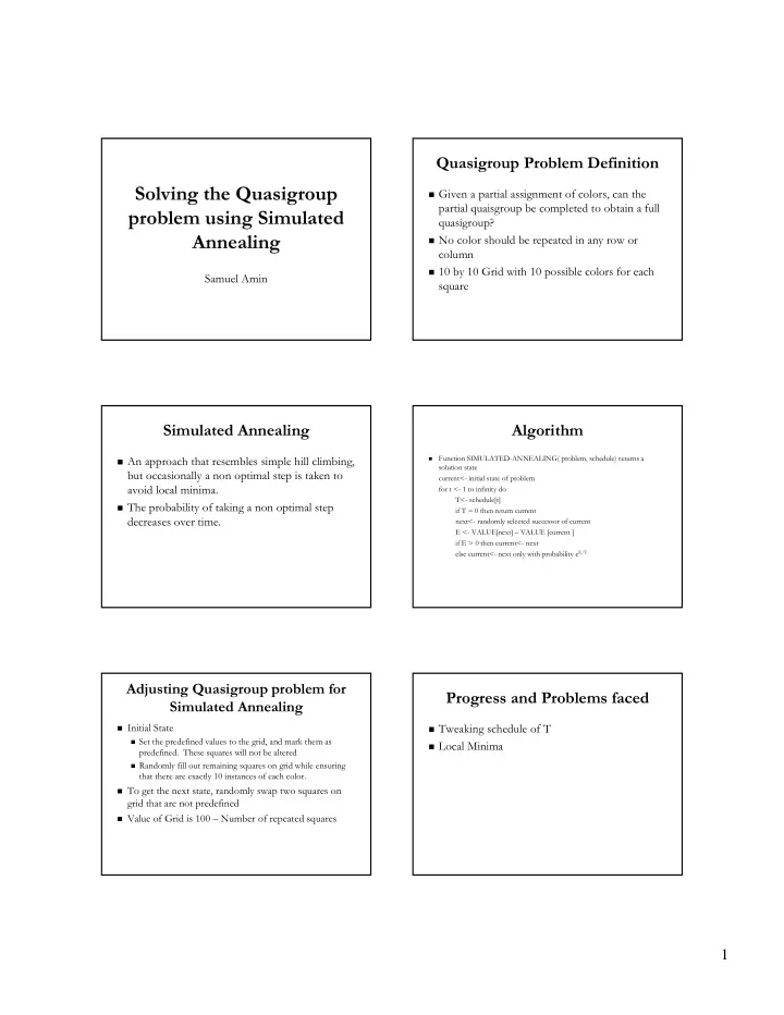
Quasigroup Problem Definition Problem Definition Quasigroup Solving the Quasigroup Solving the Quasigroup ! Given a partial assignment of colors, can the Given a partial assignment of colors, can the ! partial partial quaisgroup quaisgroup


  1. Quasigroup Problem Definition Problem Definition Quasigroup Solving the Quasigroup Solving the Quasigroup ! Given a partial assignment of colors, can the Given a partial assignment of colors, can the ! partial partial quaisgroup quaisgroup be completed to obtain a full be completed to obtain a full problem using Simulated problem using Simulated quasigroup quasigroup? ? Annealing Annealing ! No color should be repeated in any row or No color should be repeated in any row or ! column column ! 10 by 10 Grid with 10 possible colors for each 10 by 10 Grid with 10 possible colors for each ! Samuel Amin Samuel Amin square square Simulated Annealing Algorithm Simulated Annealing Algorithm ! An approach that resembles simple hill climbing, An approach that resembles simple hill climbing, Function SIMULATED- Function SIMULATED -ANNEALING( problem, schedule) returns a ANNEALING( problem, schedule) returns a ! ! ! solution state solution state but occasionally a non optimal step is taken to but occasionally a non optimal step is taken to current<- - initial state of problem initial state of problem current< avoid local minima. avoid local minima. for t < for t <- - 1 to infinity do 1 to infinity do T<- - schedule[t schedule[t] ] T< ! The probability of taking a non optimal step The probability of taking a non optimal step ! if T = 0 then return current if T = 0 then return current decreases over time. decreases over time. next< next<- - randomly selected successor of current randomly selected successor of current E < E <- - VALUE[next VALUE[next] ] – – VALUE [current ] VALUE [current ] if E > 0 then current< if E > 0 then current<- - next next else current<- - next only with probability next only with probability e e E E/T /T else current< Adjusting Quasigroup Adjusting Quasigroup problem for problem for Progress and Problems faced Progress and Problems faced Simulated Annealing Simulated Annealing ! Initial State Initial State ! Tweaking schedule of T Tweaking schedule of T ! ! ! Set the predefined values to the grid, and mark them as Set the predefined values to the grid, and mark them as ! ! Local Minima Local Minima ! predefined. These squares will not be altered predefined. These squares will not be altered ! Randomly fill out remaining squares on grid while ensuring Randomly fill out remaining squares on grid while ensuring ! that there are exactly 10 instances of each color. that there are exactly 10 instances of each color. ! To get the next state, randomly swap two squares on To get the next state, randomly swap two squares on ! grid that are not predefined grid that are not predefined ! Value of Grid is 100 Value of Grid is 100 – – Number of repeated squares Number of repeated squares ! 1

  2. System Architecture System Architecture Handwritten Character Handwritten Character Recognition using Neural Recognition using Neural • Image (bitmap) Object • Image (bitmap) Object – 16x16 bitmap scaling – 16x16 bitmap scaling Networks Networks – I/O I/O – • Neural network object • Neural network object – Training and learning Training and learning – – – Recognition Recognition • User interface • User interface CSE 592 Project CSE 592 Project – – Hand Hand- -write characters write characters Samer Arafeh Samer Arafeh – – Controls learning rate Controls learning rate – Save learned data – Save learned data Neural Network Neural Network Network nodes evaluation Network nodes evaluation • Multi • • 256 input nodes: 0.5 if pixel is on, • Multi- -layer: 3 Layers neural network layer: 3 Layers neural network 256 input nodes: 0.5 if pixel is on, otherwise - otherwise -0.5. 0.5. - 256 Input nodes (node for each for each 256 Input nodes (node for each for each - • Hidden nodes and output nodes are • input pixel) Hidden nodes and output nodes are input pixel) calculated using the sigmoid threshold unit calculated using the sigmoid threshold unit - variable number of hidden nodes - variable number of hidden nodes as: as: (currently set to 25) (currently set to 25) o = 1/(1+e - ) where o = 1/(1+e -net net ) where - 36 output nodes (0 - 36 output nodes (0- -9 and ‘A’ to ‘Z’) 9 and ‘A’ to ‘Z’) net = ∑ w net = ∑ w i i x x i (over all incoming edges) (over all incoming edges) i Backpropagation Training Backpropagation Training • • Hidden and Output weights are initialized to • For each hidden node, re • Hidden and Output weights are initialized to For each hidden node, re- -evaluate each of evaluate each of random values between [- random values between [ -0.5,0.5] 0.5,0.5] the output node weight edges (w the output node weight edges (w newo newo ) as: ) as: • For each output node, calculate the error term • For each output node, calculate the error term w newo = w oldo + ( η δ η δ k h) ; ) ; h is the hidden node value, w newo = w oldo + ( k h δ k as: δ k as: h is the hidden node value, η η is the learning rate is the learning rate δ k δ k = (t = (t k k – – o o k k ) ) • Back propagate the error term to the hidden • Back propagate the error term to the hidden • For each input node, re • For each input node, re- -evaluate each of evaluate each of nodes such that, for each hidden node, calculate nodes such that, for each hidden node, calculate the hidden node weight edges (w newh ) as: the hidden node weight edges (w newh ) as: the error term δ the error term δ h h as: as: w w newh newh = w = w oldh oldh + ( + ( η δ η δ h h x x) ; ) ; x is the input node value, δ h δ h = ∑ w = ∑ w kh kh δ δ k k (over all hidden node edges) (over all hidden node edges) x is the input node value, η η is the learning rate is the learning rate 2

  3. Recognition Recognition • Run the re • Run the re- -evalaution algorithm again with evalaution algorithm again with the new set of weighted edges and find the new set of weighted edges and find the output node with the largest which the output node with the largest which Demo Demo would correspond to the recognized would correspond to the recognized character. character. IBM ’s Robocode an AI Playground Rob ocod e ! IBM’s RoboCode ! Virtual platform to test AI concepts ! Little tanks battle each other ! Each tank has a gun and radar ! Each tank is allotted the same by Diana Bullion resources (energy, ammunition) Robots Battle ! Built 5 Robots with different strategies – Diana’s First …simple tutorial-like robot – BumperBot …brute force tank – ThirdTimeCharmer …focused attack – TheGreatX …stays out of the way – MasterEvader … predicts aiming point ! Implement multiple robots with varying levels of intelligence ! Wanted to prove intelligence and strategy wins over brute force 3

  4. BumperBot MasterEvader ! Basic robot scans for other robots ! Advanced Robot ! Bumps into them and repeatedly shoots ! Evasive Movements … random figure-eight ish pattern ! Brute force - low intelligence ! Predicts best path to fire bullet … taking – Does not predict where robot will be into account future speed and location – Does not stay focused on closest robot of both target and source robots, time to when different robot is scanned turn gun, time for bullet to travel ! Results were surprising - original objective was for the more intelligent ! Fire power relative to target distance robots to win against BumperBot Results The Rest ! ThirdTimeCharmer – Advanced Robot – Maintains a focused attack – Standard movement pattern ! Survival – 50 pts for everyone that died before it ! TheGreatX ! Last Survivor – 10 pts for every robot in battle ! Bullet Damage – 1 pt for each pt of inflicted damage – Travels great distances ! Bullet Damage Bonus – 20% kill bonus of all the – Rarely shoots damage it did – Lets others run out of energy ! Ram Damage – 2 pts for every pt of ram damage ! Diana’s First ! Ram Damage Bonus – 30% kill bonus of all ram damage it did – My first robot … modified tutorial Robocode Rules ! Evironment loop – Robot code executed, time incremented, Learning Go with TD( λ ) bullets move, robots move, robots scan ! Bullets – Bullet damage = 4*firepower (plus Todd Detwiler 2*(firepower-1) if firepower > 1) CSE 592 – Bullet speed = 20 – 3*firepower Winter 2003 – Energy returned on hit = 3 * firepower ! Robot Collision = .6 damage each ! Advanced Robots take Wall Collision penalty 4

Download Presentation
Download Policy: The content available on the website is offered to you 'AS IS' for your personal information and use only. It cannot be commercialized, licensed, or distributed on other websites without prior consent from the author. To download a presentation, simply click this link. If you encounter any difficulties during the download process, it's possible that the publisher has removed the file from their server.

Recommend


More recommend