Problem-solving agents function Simple-Problem-Solving-Agent ( - - PowerPoint PPT Presentation

problem solving agents
SMART_READER_LITE
LIVE PREVIEW

Problem-solving agents function Simple-Problem-Solving-Agent ( - - PowerPoint PPT Presentation

Problem-solving agents function Simple-Problem-Solving-Agent ( percept ) returns an action static : seq , an action sequence, initially empty state , some description of the current world state Solving Problems by Searching goal , a goal, initially


slide-1
SLIDE 1

Solving Problems by Searching

Chapter 3

Chapter 3 1

Outline

♦ Problem-solving agents ♦ Problem types ♦ Problem formulation ♦ Example problems ♦ Basic search algorithms

Chapter 3 2

Problem-solving agents

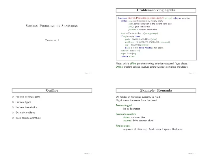
function Simple-Problem-Solving-Agent( percept) returns an action static: seq, an action sequence, initially empty state, some description of the current world state goal, a goal, initially null problem, a problem formulation state ← Update-State(state, percept) if seq is empty then goal ← Formulate-Goal(state) problem ← Formulate-Problem(state, goal) seq ← Search( problem) if seq is failure then return a null action action ← First(seq) seq ← Rest(seq) return action

Note: this is offline problem solving; solution executed “eyes closed.” Online problem solving involves acting without complete knowledge.

Chapter 3 3

Example: Romania

On holiday in Romania; currently in Arad. Flight leaves tomorrow from Bucharest Formulate goal: be in Bucharest Formulate problem: states: various cities actions: drive between cities Find solution: sequence of cities, e.g., Arad, Sibiu, Fagaras, Bucharest

Chapter 3 4

slide-2
SLIDE 2

Example: Romania

Giurgiu Urziceni Hirsova Eforie Neamt Oradea Zerind Arad Timisoara Lugoj Mehadia Dobreta Craiova Sibiu Fagaras Pitesti Vaslui Iasi Rimnicu Vilcea Bucharest 71 75 118 111 70 75 120 151 140 99 80 97 101 211 138 146 85 90 98 142 92 87 86

Chapter 3 5

Problem types

Deterministic, fully observable = ⇒ single-state problem Agent knows exactly which state it will be in; solution is a sequence Non-observable = ⇒ conformant problem Agent may have no idea where it is; solution (if any) is a sequence Nondeterministic and/or partially observable = ⇒ contingency problem percepts provide new information about current state solution is a contingent plan or a policy

  • ften interleave search, execution

Unknown state space = ⇒ exploration problem (“online”)

Chapter 3 6

Example: vacuum world

Single-state, start in #5. Solution??

1 2 3 4 5 6 7 8

Chapter 3 7

Example: vacuum world

Single-state, start in #5. Solution?? [Right, Suck] Conformant, start in {1, 2, 3, 4, 5, 6, 7, 8} e.g., Right goes to {2, 4, 6, 8}. Solution??

1 2 3 4 5 6 7 8

Chapter 3 8

slide-3
SLIDE 3

Example: vacuum world

Single-state, start in #5. Solution?? [Right, Suck] Conformant, start in {1, 2, 3, 4, 5, 6, 7, 8} e.g., Right goes to {2, 4, 6, 8}. Solution?? [Right, Suck, Left, Suck] Contingency ♦ Murphy’s Law (non-deterministic): Suck can dirty a clean carpet; start in #5 ♦ Local sensing (partially-observable): dirt, location only, start in {#5,#7}. Solution??

1 2 3 4 5 6 7 8

Chapter 3 9

Example: vacuum world

Single-state, start in #5. Solution?? [Right, Suck] Conformant, start in {1, 2, 3, 4, 5, 6, 7, 8} e.g., Right goes to {2, 4, 6, 8}. Solution?? [Right, Suck, Left, Suck] Contingency ♦ Murphy’s Law (non-deterministic): Suck can dirty a clean carpet; start in #5 ♦ Local sensing (partially-observable): dirt, location only, start in {#5,#7}. Solution?? [Right, while dirt do Suck] [Right, if dirt then Suck]

1 2 3 4 5 6 7 8

Chapter 3 10

Single-state problem formulation

A problem is defined by four items: ♦ initial state e.g., “at Arad” ♦ successor function S(x) = set of action–state pairs e.g., S(Arad) = {Arad → Zerind, Zerind, . . .} ♦ goal test, can be explicit, e.g., x = “at Bucharest” implicit, e.g., NoDirt(x) ♦ path cost (additive) e.g., sum of distances, number of actions executed, etc. c(x, a, y) is the step cost, assumed to be ≥ 0 A solution is a sequence of actions leading from the initial state to a goal state

Chapter 3 11

Selecting a state space

Real world is absurdly complex ⇒ state space must be abstracted for problem solving ♦ (Abstract) state = set of real states ♦ (Abstract) action = complex combination of real actions e.g., “Arad → Zerind” represents a complex set

  • f possible routes, detours, rest stops, etc.

♦ For guaranteed realizability, any real state “in Arad” must get to some real state “in Zerind” ♦ (Abstract) solution = set of real paths that are solutions in the real world ♦ Each abstract action should be “easier” than the original problem!

Chapter 3 12

slide-4
SLIDE 4

Example: vacuum world state space graph

R L S S S S R L R L R L S S S S L L L L R R R R

states?? actions?? goal test?? path cost??

Chapter 3 13

Example: vacuum world state space graph

R L S S S S R L R L R L S S S S L L L L R R R R

states??: integer dirt and robot locations (ignore dirt amounts etc.) actions?? goal test?? path cost??

Chapter 3 14

Example: vacuum world state space graph

R L S S S S R L R L R L S S S S L L L L R R R R

states??: integer dirt and robot locations (ignore dirt amounts etc.) actions??: Left, Right, Suck, NoOp goal test?? path cost??

Chapter 3 15

Example: vacuum world state space graph

R L S S S S R L R L R L S S S S L L L L R R R R

states??: integer dirt and robot locations (ignore dirt amounts etc.) actions??: Left, Right, Suck, NoOp goal test??: no dirt path cost??

Chapter 3 16

slide-5
SLIDE 5

Example: vacuum world state space graph

R L S S S S R L R L R L S S S S L L L L R R R R

states??: integer dirt and robot locations (ignore dirt amounts etc.) actions??: Left, Right, Suck, NoOp goal test??: no dirt path cost??: 1 per action (0 for NoOp)

Chapter 3 17

Example: The 8-puzzle

2

Start State Goal State

5 1 3 4 6 7 8 5 1 2 3 4 6 7 8 5

states?? actions?? goal test?? path cost??

Chapter 3 18

Example: The 8-puzzle

2

Start State Goal State

5 1 3 4 6 7 8 5 1 2 3 4 6 7 8 5

states??: integer locations of tiles (ignore intermediate positions) actions?? goal test?? path cost??

Chapter 3 19

Example: The 8-puzzle

2

Start State Goal State

5 1 3 4 6 7 8 5 1 2 3 4 6 7 8 5

states??: integer locations of tiles (ignore intermediate positions) actions??: move blank left, right, up, down (ignore unjamming etc.) goal test?? path cost??

Chapter 3 20

slide-6
SLIDE 6

Example: The 8-puzzle

2

Start State Goal State

5 1 3 4 6 7 8 5 1 2 3 4 6 7 8 5

states??: integer locations of tiles (ignore intermediate positions) actions??: move blank left, right, up, down (ignore unjamming etc.) goal test??: = goal state (given) path cost??

Chapter 3 21

Example: The 8-puzzle

2

Start State Goal State

5 1 3 4 6 7 8 5 1 2 3 4 6 7 8 5

states??: integer locations of tiles (ignore intermediate positions) actions??: move blank left, right, up, down (ignore unjamming etc.) goal test??: = goal state (given) path cost??: 1 per move [Note: optimal solution of n-Puzzle family is NP-hard]

Chapter 3 22

Example: robotic assembly

R R R P R R

states??: real-valued coordinates of robot joint angles parts of the object to be assembled actions??: continuous motions of robot joints goal test??: complete assembly with no robot included! path cost??: time to execute

Chapter 3 23

Tree search algorithms

Basic idea:

  • ffline, simulated exploration of state space

by generating successors of already-explored states (a.k.a. expanding states)

function Tree-Search( problem, strategy) returns a solution, or failure initialize the frontier using the initial state of problem loop do if the frontier is empty then return failure choose a leaf node and remove it from the frontier based on strategy if the node contains a goal state then return the corresponding solution else expand the chosen node and add the resulting nodes to the frontier end

Chapter 3 24

slide-7
SLIDE 7

Tree search example

Rimnicu Vilcea

Lugoj Zerind Sibiu Arad Fagaras Oradea Timisoara Arad Arad Oradea Arad

Chapter 3 25

Tree search example

Rimnicu Vilcea

Lugoj Arad Fagaras Oradea Arad Arad Oradea Zerind Arad Sibiu Timisoara

Chapter 3 26

Tree search example

Lugoj Arad Arad Oradea

Rimnicu Vilcea

Zerind Arad Sibiu Arad Fagaras Oradea Timisoara

Chapter 3 27

Implementation: states vs. nodes

A state is a (representation of) a physical configuration A node is a data structure constituting part of a search tree includes parent, children, depth, path cost g(x) States do not have parents, children, depth, or path cost!

1 2 3 4 5 6 7 8 1 2 3 4 5 6 7 8

State Node

depth = 6 g = 6 state parent, action

The Expand function creates new nodes, filling in the various fields and using the SuccessorFn of the problem to create the corresponding states.

Chapter 3 28

slide-8
SLIDE 8

Search strategies

A strategy is defined by picking the order of node expansion Strategies are evaluated along the following dimensions: completeness—does it always find a solution if one exists? time complexity—number of nodes generated/expanded space complexity—maximum number of nodes in memory

  • ptimality—does it always find a least-cost solution?

Time and space complexity are measured in terms of b—maximum branching factor of the search tree d—depth of the “shallowest” solution m—maximum depth of the state space (may be ∞)

Chapter 3 29

Uninformed search strategies

Uninformed strategies use only the information available in the problem definition ♦ Breadth-first search ♦ Uniform-cost search ♦ Depth-first search ♦ Depth-limited search ♦ Iterative deepening search

Chapter 3 30

Breadth-first search

Expand shallowest unexpanded node Implementation: frontier is a FIFO queue, i.e., new successors go at end

A B C D E F G

Chapter 3 31

Breadth-first search

Expand shallowest unexpanded node Implementation: frontier is a FIFO queue, i.e., new successors go at end

A B C D E F G

Chapter 3 32

slide-9
SLIDE 9

Breadth-first search

Expand shallowest unexpanded node Implementation: frontier is a FIFO queue, i.e., new successors go at end

A B C D E F G

Chapter 3 33

Breadth-first search

Expand shallowest unexpanded node Implementation: frontier is a FIFO queue, i.e., new successors go at end

A B C D E F G

Chapter 3 34

Properties of breadth-first search

Complete??

Chapter 3 35

Properties of breadth-first search

Complete?? Yes (if b is finite) Time??

Chapter 3 36

slide-10
SLIDE 10

Properties of breadth-first search

Complete?? Yes (if b is finite) Time (# of visited nodes)?? 1 + b + b2 + b3 + . . . + bd = O(bd) Time (# of generated nodes)?? b+b2+b3+. . .+bd+(bd+1−b) = O(bd+1) Space??

Chapter 3 37

Properties of breadth-first search

Complete?? Yes (if b is finite) Time (# of generated nodes)?? b+b2+b3+. . .+bd+(bd+1−b) = O(bd+1) Space?? O(bd+1) (keeps every node in memory) Optimal??

Chapter 3 38

Properties of breadth-first search

Complete?? Yes (if b is finite) Time (# of generated nodes)?? b+b2+b3+. . .+bd+(bd+1−b) = O(bd+1) Space?? O(bd+1) (keeps every node in memory) Optimal?? Yes (if cost = 1 per step); not optimal in general Space is the big problem; can easily generate nodes at 100MB/sec so 24hrs = 8640GB.

Chapter 3 39

Uniform-cost search

Expand least-cost unexpanded node Implementation: frontier = queue ordered by path cost, lowest first Equivalent to breadth-first if step costs all equal Complete?? Yes, if step cost ≥ ǫ (lowest step cost) Time?? # of nodes with g ≤ cost of optimal solution, O(b⌈C∗/ǫ⌉) where C∗ is the cost of the optimal solution Space?? # of nodes with g ≤ cost of optimal solution, O(b⌈C∗/ǫ⌉) Optimal?? Yes—nodes expanded in increasing order of g(n)

Chapter 3 40

slide-11
SLIDE 11

Depth-first search

Expand deepest unexpanded node Implementation: frontier = LIFO queue, i.e., put successors at front

A B C D E F G H I J K L M N O

Chapter 3 41

Depth-first search

Expand deepest unexpanded node Implementation: frontier = LIFO queue, i.e., put successors at front

A B C D E F G H I J K L M N O

Chapter 3 42

Depth-first search

Expand deepest unexpanded node Implementation: frontier = LIFO queue, i.e., put successors at front

A B C D E F G H I J K L M N O

Chapter 3 43

Depth-first search

Expand deepest unexpanded node Implementation: frontier = LIFO queue, i.e., put successors at front

A B C D E F G H I J K L M N O

Chapter 3 44

slide-12
SLIDE 12

Depth-first search

Expand deepest unexpanded node Implementation: frontier = LIFO queue, i.e., put successors at front

A B C D E F G H I J K L M N O

Chapter 3 45

Depth-first search

Expand deepest unexpanded node Implementation: frontier = LIFO queue, i.e., put successors at front

A B C D E F G H I J K L M N O

Chapter 3 46

Depth-first search

Expand deepest unexpanded node Implementation: frontier = LIFO queue, i.e., put successors at front

A B C D E F G H I J K L M N O

Chapter 3 47

Depth-first search

Expand deepest unexpanded node Implementation: frontier = LIFO queue, i.e., put successors at front

A B C D E F G H I J K L M N O

Chapter 3 48

slide-13
SLIDE 13

Depth-first search

Expand deepest unexpanded node Implementation: frontier = LIFO queue, i.e., put successors at front

A B C D E F G H I J K L M N O

Chapter 3 49

Depth-first search

Expand deepest unexpanded node Implementation: frontier = LIFO queue, i.e., put successors at front

A B C D E F G H I J K L M N O

Chapter 3 50

Depth-first search

Expand deepest unexpanded node Implementation: frontier = LIFO queue, i.e., put successors at front

A B C D E F G H I J K L M N O

Chapter 3 51

Depth-first search

Expand deepest unexpanded node Implementation: frontier = LIFO queue, i.e., put successors at front

A B C D E F G H I J K L M N O

Chapter 3 52

slide-14
SLIDE 14

Properties of depth-first search

Complete??

Chapter 3 53

Properties of depth-first search

Complete?? Yes: in finite spaces No: fails in infinite-depth spaces, spaces with loops Modify to avoid repeated states along path Time??

Chapter 3 54

Properties of depth-first search

Complete?? Yes: in finite spaces No: fails in infinite-depth spaces, spaces with loops Modify to avoid repeated states along path Time?? O(bm): terrible if m is much larger than d but if solutions are dense, may be much faster than breadth-first Space??

Chapter 3 55

Properties of depth-first search

Complete?? Yes: in finite spaces No: fails in infinite-depth spaces, spaces with loops Modify to avoid repeated states along path Time?? O(bm): terrible if m is much larger than d but if solutions are dense, may be much faster than breadth-first Space?? O(bm), i.e., linear space! Optimal??

Chapter 3 56

slide-15
SLIDE 15

Properties of depth-first search

Complete?? Yes: in finite spaces No: fails in infinite-depth spaces, spaces with loops Modify to avoid repeated states along path Time?? O(bm): terrible if m is much larger than d but if solutions are dense, may be much faster than breadth-first Space?? O(bm), i.e., linear space! Optimal?? No

Chapter 3 57

Depth-limited search

= depth-first search with depth limit l, i.e., nodes at depth l have no successors Recursive implementation:

function Depth-Limited-Search( problem,limit) returns soln/fail/cutoff Recursive-DLS(Make-Node(Initial-State[problem]),problem,limit) function Recursive-DLS(node,problem,limit) returns soln/fail/cutoff cutoff-occurred? ← false if Goal-Test(problem,State[node]) then return node else if Depth[node] = limit then return cutoff else for each successor in Expand(node,problem) do result ← Recursive-DLS(successor,problem,limit) if result = cutoff then cutoff-occurred? ← true else if result = failure then return result if cutoff-occurred? then return cutoff else return failure

Chapter 3 58

Iterative deepening search

function Iterative-Deepening-Search( problem) returns a solution inputs: problem, a problem for depth ← 0 to ∞ do result ← Depth-Limited-Search( problem, depth) if result = cutoff then return result end

Chapter 3 59

Iterative deepening search l = 0

Limit = 0

A A Chapter 3 60

slide-16
SLIDE 16

Iterative deepening search l = 1

Limit = 1

A B C A B C A B C A B C Chapter 3 61

Iterative deepening search l = 2

Limit = 2

A B C D E F G A B C D E F G A B C D E F G A B C D E F G A B C D E F G A B C D E F G A B C D E F G A B C D E F G Chapter 3 62

Iterative deepening search l = 3

Limit = 3

A B C D E F G H I J K L M N O A B C D E F G H I J K L M N O A B C D E F G H I J K L M N O A B C D E F G H I J K L M N O A B C D E F G H I J K L M N O A B C D E F G H I J K L M N O A B C D E F G H I J K L M N O A B C D E F G H I J K L M N O A B C D E F G H I J K L M N O A B C D E F G H I J K L M N O A B C D E F G H J K L M N O I A B C D E F G H I J K L M N O Chapter 3 63

Properties of iterative deepening search

Complete??

Chapter 3 64

slide-17
SLIDE 17

Properties of iterative deepening search

Complete?? Yes Time??

Chapter 3 65

Properties of iterative deepening search

Complete?? Yes Time (# of generated nodes)?? db1 + (d − 1)b2 + . . . + bd = O(bd) Space??

Chapter 3 66

Properties of iterative deepening search

Complete?? Yes Time (# of generated nodes)?? db1 + (d − 1)b2 + . . . + bd = O(bd) Space?? O(bd) Optimal??

Chapter 3 67

Properties of iterative deepening search

Complete?? Yes Time (# of generated nodes)?? db1 + (d − 1)b2 + . . . + bd = O(bd) Space?? O(bd) Optimal?? Yes, if step cost = 1 Can be modified to explore uniform-cost tree Numerical comparison for b = 10 and d = 5, solution at far right leaf: N(IDS) = 50 + 400 + 3, 000 + 20, 000 + 100, 000 = 123, 450 Nvisited(BFS) = 10 + 100 + 1, 000 + 10, 000 + 100, 000 = 111, 110 Ngenerated(BFS) = 10 + 100 + 1, 000 + 10, 000 + 100, 000 + 999, 990 = 1, 111, 100 BFS can be modified to apply goal test when a node is generated

Chapter 3 68

slide-18
SLIDE 18

Summary of algorithms

Criterion Breadth- Uniform- Depth- Depth- Iterative First Cost First Limited Deepening Complete? Yes Yes No Yes, if l ≥ d Yes Time (big-O) bd b⌈C∗/ǫ⌉ bm bl bd Space (big-O) bd b⌈C∗/ǫ⌉ bm bl bd Optimal? Yes∗ Yes No No Yes∗

Chapter 3 69

Repeated states

Failure to detect repeated states can turn a linear problem into an exponential

  • ne!

A B C D A B B C C C C

Chapter 3 70

Graph search

function Graph-Search( problem) returns a solution, or failure frontier ← a list with node from the initial state of problem explored ← an empty set loop do if frontier is empty then return failure node ← Remove-Front(frontier) if node contains a goal state then return Solution(node) add State[node] to explored expand node add to frontier the resulting nodes that are not in explored or not in frontier or [better than the corresponding nodes in frontier in some algs] end

frontier (aka fringe or open); explored (aka visited or closed)

Chapter 3 71

Informed Search

♦ So far the search algorithms are “uninformed”—independent to the prob- lems ♦ Informed search–incorporating knowledge related to the problem for guid- ing search

Chapter 3 72

slide-19
SLIDE 19

Best-first search

Idea: use an evaluation function for each node – estimate of “desirability” ⇒ Expand most desirable unexpanded node Implementation: frontier is a queue sorted in decreasing order of desirability Special cases: greedy search A∗ search

Chapter 3 73

Romania with step costs in km

Bucharest Giurgiu Urziceni Hirsova Eforie Neamt Oradea Zerind Arad Timisoara Lugoj Mehadia Dobreta Craiova Sibiu Fagaras Pitesti Rimnicu Vilcea Vaslui Iasi Straight−line distance to Bucharest 160 242 161 77 151 241 366 193 178 253 329 80 199 244 380 226 234 374 98

Giurgiu Urziceni Hirsova Eforie Neamt Oradea Zerind Arad Timisoara Lugoj Mehadia Dobreta Craiova Sibiu Fagaras Pitesti Vaslui Iasi Rimnicu Vilcea Bucharest

71 75 118 111 70 75 120 151 140 99 80 97 101 211 138 146 85 90 98 142 92 87 86

Chapter 3 74

Greedy search

Evaluation function h(n) (heuristic) = estimate of cost from n to the closest goal E.g., hSLD(n) = straight-line distance from n to Bucharest Greedy search expands the node that appears to be closest to goal

Chapter 3 75

Greedy search example

Arad 366

Chapter 3 76

slide-20
SLIDE 20

Greedy search example

Zerind Arad Sibiu Timisoara 253 329 374

Chapter 3 77

Greedy search example

Rimnicu Vilcea

Zerind Arad Sibiu Arad Fagaras Oradea Timisoara 329 374 366 176 380 193

Chapter 3 78

Greedy search example

Rimnicu Vilcea

Zerind Arad Sibiu Arad Fagaras Oradea Timisoara Sibiu Bucharest 329 374 366 380 193 253

Chapter 3 79

Properties of greedy search

Complete??

Chapter 3 80

slide-21
SLIDE 21

Properties of greedy search

Complete?? Yes–Complete in finite space with repeated-state checking No–can get stuck in loops, e.g., with Oradea as goal, Iasi → Neamt → Iasi → Neamt → Time??

Chapter 3 81

Properties of greedy search

Complete?? Yes–Complete in finite space with repeated-state checking No–can get stuck in loops, e.g., Iasi → Neamt → Iasi → Neamt → Time?? O(bm), but a good heuristic can give dramatic improvement Space??

Chapter 3 82

Properties of greedy search

Complete?? Yes–Complete in finite space with repeated-state checking No–can get stuck in loops, e.g., Iasi → Neamt → Iasi → Neamt → Time?? O(bm), but a good heuristic can give dramatic improvement Space?? O(bm), but a good heuristic can give dramatic improvement Optimal??

Chapter 3 83

Properties of greedy search

Complete?? Yes–Complete in finite space with repeated-state checking No–can get stuck in loops, e.g., Iasi → Neamt → Iasi → Neamt → Time?? O(bm), but a good heuristic can give dramatic improvement Space?? O(bm), but a good heuristic can give dramatic improvement Optimal?? No

Chapter 3 84

slide-22
SLIDE 22

A∗ search

Idea: avoid expanding paths that are already expensive Evaluation function f(n) = g(n) + h(n) g(n) = cost so far to reach n h(n) = estimated cost to goal from n f(n) = estimated total cost of path through n to goal A∗ search uses an admissible heuristic i.e., h(n) ≤ h∗(n) where h∗(n) is the true cost from n. (Also require h(n) ≥ 0, so h(G) = 0 for any goal G.) E.g., hSLD(n) never overestimates the actual road distance Theorem: A∗ search is optimal

Chapter 3 85

A∗ search example

Arad 366=0+366

Chapter 3 86

A∗ search example

Zerind Arad Sibiu Timisoara 447=118+329 449=75+374 393=140+253

Chapter 3 87

A∗ search example

Zerind Arad Sibiu Arad Timisoara

Rimnicu Vilcea

Fagaras Oradea 447=118+329 449=75+374 646=280+366 413=220+193 415=239+176 671=291+380

Chapter 3 88

slide-23
SLIDE 23

A∗ search example

Zerind Arad Sibiu Arad Timisoara Fagaras Oradea 447=118+329 449=75+374 646=280+366 415=239+176

Rimnicu Vilcea

Craiova Pitesti Sibiu 526=366+160 553=300+253 417=317+100 671=291+380

Chapter 3 89

A∗ search example

Zerind Arad Sibiu Arad Timisoara Sibiu Bucharest

Rimnicu Vilcea

Fagaras Oradea Craiova Pitesti Sibiu 447=118+329 449=75+374 646=280+366 591=338+253 450=450+0 526=366+160 553=300+253 417=317+100 671=291+380

Chapter 3 90

A∗ search example

Zerind Arad Sibiu Arad Timisoara Sibiu Bucharest

Rimnicu Vilcea

Fagaras Oradea Craiova Pitesti Sibiu Bucharest Craiova

Rimnicu Vilcea

418=418+0 447=118+329 449=75+374 646=280+366 591=338+253 450=450+0 526=366+160 553=300+253 615=455+160 607=414+193 671=291+380

Chapter 3 91

Optimality of A∗ (standard proof)

Suppose some suboptimal goal G2 has been generated and is in the queue. Let n be an unexpanded node on a shortest path to an optimal goal G.

G n G2 Start

Want to prove: f(G2) > f(n) [A∗ will never select G2 for expansion] f(G2) = g(G2) since h(G2) = 0 g(G2) > g(G) since G2 is suboptimal g(G) ≥ f(n) since h is admissible

Chapter 3 92

slide-24
SLIDE 24

Properties of A∗

Complete??

Chapter 3 93

Properties of A∗

Complete?? Yes, unless there are infinitely many nodes with f ≤ f(G) Time??

Chapter 3 94

Properties of A∗

Complete?? Yes, unless there are infinitely many nodes with f ≤ f(G) Time?? Exponential in [relative error in h × d] Space??

Chapter 3 95

Properties of A∗

Complete?? Yes, unless there are infinitely many nodes with f ≤ f(G) Time?? Exponential in [relative error in h × d] Space?? Exponential Optimal??

Chapter 3 96

slide-25
SLIDE 25

Properties of A∗

Complete?? Yes, unless there are infinitely many nodes with f ≤ f(G) Time?? Exponential in [relative error in h × d] Space?? Exponential Optimal?? Yes—cannot expand fi+1 until fi is finished, where fi+1 > fi C∗ is the cost for the optimal solution: A∗ expands all nodes with f(n) < C∗ A∗ expands some nodes with f(n) = C∗ A∗ expands no nodes with f(n) > C∗

Chapter 3 97

A* vs Uniform-cost Search

f(n) = g(n) + h(n) Isn’t UCS just A* with h(n) being zero (admissible)? Both are optimal, why is A* usually “faster?”

Chapter 3 98

A* vs Uniform-cost Search

f(n) = g(n) + h(n) Isn’t UCS just A* with h(n) being zero (admissible)? Both are optimal, why is A* usually “faster?” Consider h(n) is perfect, f(n) is ?

Chapter 3 99

A* vs Uniform-cost Search

f(n) = g(n) + h(n) Isn’t UCS just A* with h(n) being zero (admissible)? Both are optimal, why is A* usually “faster?” Consider h(n) is perfect, f(n) is the actual total path cost.

Chapter 3 100

slide-26
SLIDE 26

A* vs Uniform-cost Search

f(n) = g(n) + h(n) Isn’t UCS just A* with h(n) being zero (admissible)? Both are optimal, why is A* usually “faster?” Consider h(n) is perfect, f(n) is the actual total path cost.

  • If n doesn’t lead to a goal state, f(n) = ∞

– A* ? – UCS ?

Chapter 3 101

A* vs Uniform-cost Search

f(n) = g(n) + h(n) Isn’t UCS just A* with h(n) being zero (admissible)? Both are optimal, why is A* usually “faster?” Consider h(n) is perfect, f(n) is the actual total path cost.

  • If n doesn’t lead to a goal state, f(n) = ∞

– A* doesn’t explore n. – UCS doesn’t know and keeps on exploring n (and its sucessors).

  • If n doesn’t lead to the optimal goal, but n∗ does: f(n) > f(n∗)

– A* ? – UCS ?

Chapter 3 102

A* vs Uniform-cost Search

f(n) = g(n) + h(n) Isn’t UCS just A* with h(n) being zero (admissible)? Both are optimal, why is A* usually “faster?” Consider h(n) is perfect, f(n) is the actual total path cost.

  • If n doesn’t lead to a goal state, f(n) = ∞

– A* doesn’t explore n. – UCS doesn’t know and keeps on exploring n (and its sucessors).

  • If n doesn’t lead to the optimal goal, but n∗ does: f(n) > f(n∗)

– A* doesn’t explore n and *only* explores n∗ ! – UCS doesn’t know and keeps on exploring n (and its sucessors). In terms of speed, the worst case for A* is when h(n) is zero, but we don’t use h(n) = 0.

Chapter 3 103

Consistency

Consider n′ is a successor of n, a heuristic is consistent if

n c(n,a,n’) h(n’) h(n) G n’

h(n) ≤ c(n, a, n′) + h(n′), Let’s find the relationship between f(n) and f(n′): f(n′) = g(n′) + h(n′) f(n′) = g(n) + c(n, a, n′) + h(n′) f(n′) ≥ g(n) + h(n) [since h is consistent] f(n′) ≥ f(n) i.e. f(n) values for a sequence of nodes along *any* path are nondecreasing (similar to g(n) values in UCS). A* using GRAPH-SEARCH is optimal if h(n) is consistent (using a similar argument as UCS).

Chapter 3 104

slide-27
SLIDE 27

Optimality of A∗ (consistent heuristics)

Lemma: A∗ expands nodes in order of increasing f value∗ Gradually adds “f-contours” of nodes (cf. breadth-first adds layers) Contour i has all nodes with f = fi, where fi < fi+1

O Z A T L M D C R F P G B U H E V I N 380 400 420 S

Chapter 3 105

Admissible vs Consistent Heuristics

Consistency is a slightly stronger/stricter requirement than admissibility. consistentHeuristics ⊂ admissibleHeuristics Admissible heuristics are usually consistent. Not easy to concort admissible, but not consistent heuristics.

Chapter 3 106

Admissible heuristics

E.g., for the 8-puzzle: h1(n) = number of misplaced tiles h2(n) = total Manhattan distance (i.e., no. of squares from desired location of each tile)

2

Start State Goal State

5 1 3 4 6 7 8 5 1 2 3 4 6 7 8 5

h1(S) =?? h2(S) =??

Chapter 3 107

Admissible heuristics

E.g., for the 8-puzzle: h1(n) = number of misplaced tiles h2(n) = total Manhattan distance (i.e., no. of squares from desired location of each tile)

2

Start State Goal State

5 1 3 4 6 7 8 5 1 2 3 4 6 7 8 5

h1(S) =?? 6 h2(S) =?? 4+0+3+3+1+0+2+1 = 14

Chapter 3 108

slide-28
SLIDE 28

Dominance

If h2(n) ≥ h1(n) for all n (both admissible) then h2 dominates h1 and is faster for search Typical search costs: d = 14 IDS = 3,473,941 nodes A∗(h1) = 539 nodes A∗(h2) = 113 nodes d = 24 IDS ≈ 54,000,000,000 nodes A∗(h1) = 39,135 nodes A∗(h2) = 1,641 nodes Given any admissible heuristics ha, hb, h(n) = max(ha(n), hb(n)) is also admissible and dominates ha, hb

Chapter 3 109

Relaxed problems

Admissible heuristics can be derived from the exact solution cost of a relaxed version of the problem If the rules of the 8-puzzle are relaxed so that a tile can move anywhere, then h1(n) gives the shortest solution If the rules are relaxed so that a tile can move to any adjacent square, then h2(n) gives the shortest solution Key point: the optimal solution cost of a relaxed problem is no greater than the optimal solution cost of the real problem

Chapter 3 110

Relaxed problems contd.

Well-known example: travelling salesperson problem (TSP) Find the shortest tour visiting all cities exactly once Minimum spanning tree can be computed in O(n2) and is a lower bound on the shortest (open) tour

Chapter 3 111

Summary

Problem formulation usually requires abstracting away real-world details to define a state space that can feasibly be explored Variety of uninformed search strategies Iterative deepening search uses only linear space and not much more time than other uninformed algorithms Graph search can be exponentially more efficient than tree search

Chapter 3 112

slide-29
SLIDE 29

Summary

Heuristic functions estimate costs of shortest paths Good heuristics can dramatically reduce search cost Greedy best-first search expands lowest h – incomplete and not always optimal A∗ search expands lowest g + h – complete and optimal – also optimally efficient (up to tie-breaks, for forward search) Admissible heuristics can be derived from exact solution of relaxed problems

Chapter 3 113