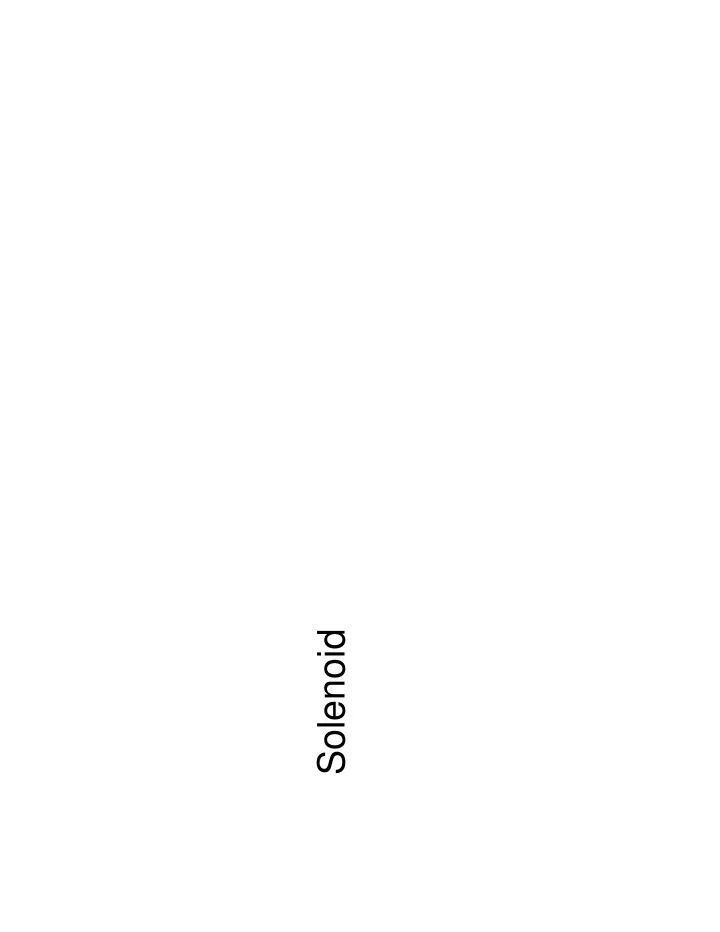
Solenoid Solenoid L I B If n = number of turns per unit length - PDF document

Solenoid

Solenoid L I B If n = number of turns per unit length        B d s B L           Ampere’s Law: B d s I B L (nL) I 0 0    B n I 0 Note that B is proportional to the number of turns per unit length, but not the total number of turns.

Toroid         B d s B 2 r Ampere’s Law:              B d s I B 2 r (n 2 r) I 0 0   N      B I  0   2 r N = Total number of turns

Structure of Equations E B Interaction between charges Interaction between moving charges/ currents      Coulomb’s Law Biot ‐ Savart Law 1 dq ˆ I d s r   ˆ 0 d E r d B   2 2 4 r 4 r 0   Gauss’s Law Gauss’s Law (Conceptual)       E d A q    0 in B d A 0   Gauss’s Law Ampere’s Law (Calculation)       E d A q     0 in B d s 0 I in Parallel capacitor gives uniform E Solenoid gives uniform B field     field   E B nI  0 0

Maxwell’s Equations Maxwell’s equations describe all the properties of electric and magnetic fields and there are four equations in it: Integral form Differential form Name of equation (optional) 1 st Equation    Electric          E d A Q E Gauss’s Law 0 enclosed 0   Magnetic       B  B d A 0 Gauss’s Law 0     Ampere’s          B d I B J Law 0 enclosed 0 (Incomplete) Not yet 2 nd Equation Lorentz force equation is not part of Maxwell’s equations. It describes what 3 rd happens when charges are put in an electric or magnetic fields:     Equation    F (q E v B )

Class 35: Faraday’s Law Part I – Maxwell’s 4 th Equation

Imaginary loop in an electric and magnetic field We will do two types of integrals for the E (non-uniform) closed loop: 1. Magnetic flux       B d A B B Note that  B  0 (Maxwell’s 2 nd equation) because this is not a 3 dimensional closed surface. Electromotive force (emf,  ) 2.       E d s loop loop  loop = 0 for electrostatic case. Note that  loop = 0 does not mean E =0.

Example I What is the magnetic flux through the rectangular loop? b d a

Old slide from class 13 Electric Potential V If E(r) is conservative, the potential difference  V is defined as the negative work done by the force F(r) (which is path independent), divided by the charge (of the test charge).  f   B     1 1 U - F ( r ) d r ` ` i Pay attention to the negative sign   f  V=0 for   U      V - E ( r ) d r 1 closed A q loop ` i Unit of electric potential = J/C =V

Old slide from class 13 Warning In the discussion here we will assume electric (force) field is a conservative (force) field. This will not be the case if there is a changing magnetic field. We will come to this point later in the semester.

Faraday’s Law – Part 1 (Maxwell’s 4 th equation) A changing magnetic field will produce an electric field and they E have the following relationship:      B  loop B t              or E d s B d A  t loop Notes: 1. We find a new way to produce an electric field. 2.  loop of electric fields produced this way does not equal to 0.