
SLIDE 1
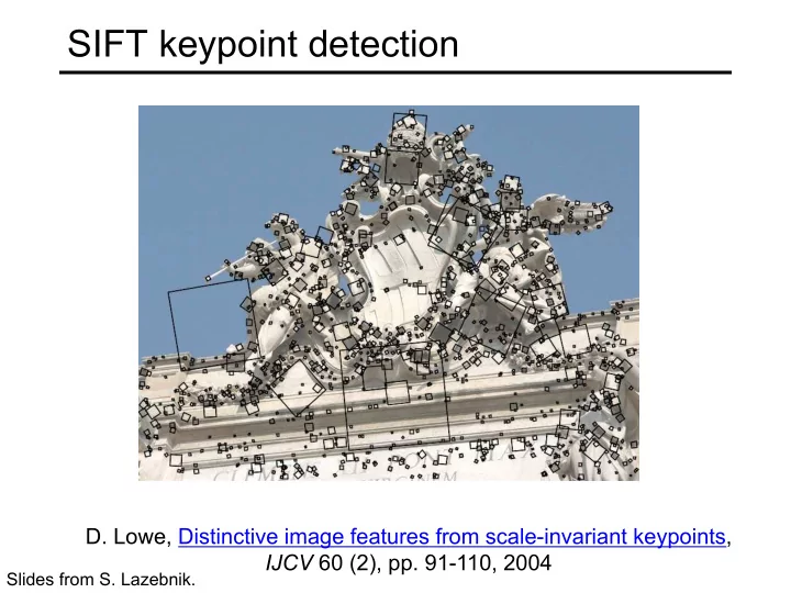
SIFT keypoint detection
- D. Lowe, Distinctive image features from scale-invariant keypoints,
IJCV 60 (2), pp. 91-110, 2004
Slides from S. Lazebnik.
SIFT keypoint detection D. Lowe, Distinctive image features from - - PowerPoint PPT Presentation
SIFT keypoint detection D. Lowe, Distinctive image features from scale-invariant keypoints, IJCV 60 (2), pp. 91-110, 2004 Slides from S. Lazebnik. Keypoint detection with scale selection We want to extract keypoints with characteristic
Slides from S. Lazebnik.
Source: L. Lazebnik
Source: L. Lazebnik
Source: N. Snavely
Source: L. Lazebnik
Source: L. Lazebnik
Source: S. Seitz
Source: L. Lazebnik
2 2
2 2
Source: S. Seitz
Source: L. Lazebnik
Source: L. Lazebnik
Source: L. Lazebnik
Source: L. Lazebnik
Source: L. Lazebnik
Source: L. Lazebnik
Source: L. Lazebnik
2 2 2
Source: L. Lazebnik
Source: L. Lazebnik
Source: L. Lazebnik
Source: L. Lazebnik
Source: L. Lazebnik
Source: L. Lazebnik
2
xx yy
Source: L. Lazebnik
Source: L. Lazebnik
Source: L. Lazebnik
Source: L. Lazebnik
Source: L. Lazebnik
2 p
Source: L. Lazebnik
Source: L. Lazebnik
Source: L. Lazebnik
Source: L. Lazebnik
– Up to about 60 degree out-of-plane rotation
– Sometimes even day vs. night
Source: N. Snavely