1 Scale space representation Scale space representation Keypoint - - PDF document

SLIDE 1

1

Distinctive Image Features from Distinctive Image Features from Scale Scale-

• Invariant

Invariant Keypoints Keypoints David G. Lowe David G. Lowe

presented by, presented by, Sudheendra Sudheendra

Introduction Introduction

• Invariance

Invariance

• Intensity

Intensity

• Scale

Scale

• Rotation

Rotation

• Affine

Affine

• View point

View point

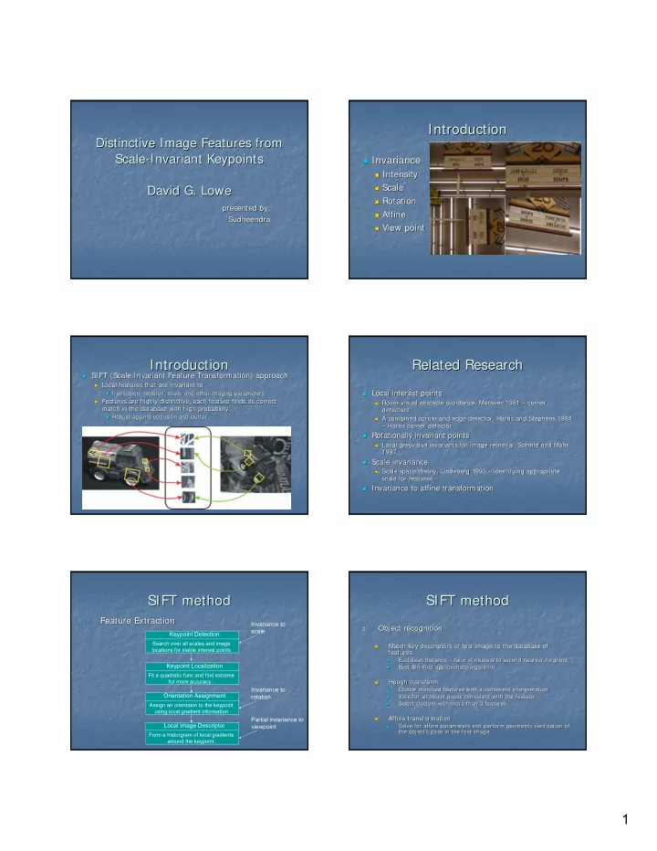
Introduction Introduction

• SIFT (Scale Invariant Feature Transformation) approach

SIFT (Scale Invariant Feature Transformation) approach

• Local features that are invariant to

Local features that are invariant to

• translation, rotation, scale, and other imaging parameters

translation, rotation, scale, and other imaging parameters

• Features are highly distinctive, each feature finds its correct

Features are highly distinctive, each feature finds its correct match in the database with high probability match in the database with high probability

• Robust against occlusion and clutter

Robust against occlusion and clutter

Related Research Related Research

• Local interest points

Local interest points

• Rover visual obstacle avoidance,

Rover visual obstacle avoidance, Moravec Moravec 1981 1981 – – corner corner detectors detectors

• A combined corner and edge detector, Harris and Stephens 1988

A combined corner and edge detector, Harris and Stephens 1988 – – Harris corner detector Harris corner detector

• Rotationally invariant points

Rotationally invariant points

• Local

Local greyvalue greyvalue invariants for image retrieval, invariants for image retrieval, Schmid Schmid and Mohr and Mohr 1997 1997

• Scale invariance

Scale invariance

• Scale space theory,

Scale space theory, Lindeberg Lindeberg 1993 1993 – – identifying appropriate identifying appropriate scale for features scale for features

• Invariance to affine transformation

Invariance to affine transformation

SIFT method SIFT method

1. 1.

Feature Extraction Feature Extraction

Keypoint Detection

Search over all scales and image locations for stable interest points

Keypoint Localization

Fit a quadratic func and find extrema for more accuracy .

Orientation Assignment

Assign an orientaion to the keypoint using local gradient information

Local image Descriptor

Form a historgram of local gradients around the keypoint.

Invariance to scale Invariance to rotation Partial invariance to viewpoint

SIFT method SIFT method

2. 2.

Object recognition Object recognition

• Match key descriptors of test image to the database of

Match key descriptors of test image to the database of features features

• Euclidean distance

Euclidean distance – – ratio of nearest to second nearest neighbor ratio of nearest to second nearest neighbor

• Best

Best-

• Bin

Bin-

• First approximate algorithm

First approximate algorithm

• Hough transform

Hough transform

• Cluster matched features with a consistent interpretation

Cluster matched features with a consistent interpretation

• Vote for all object poses consistent with the feature

Vote for all object poses consistent with the feature

• Select clusters with more than 3 features

Select clusters with more than 3 features

• Affine transformation

Affine transformation

• Solve for affine parameters and perform geometric verification o

Solve for affine parameters and perform geometric verification of f the object’s pose in the test image the object’s pose in the test image

SLIDE 2

2 Keypoint Keypoint detection detection

• Goal

Goal – – detect detect keypoints keypoints that are invariant to scale that are invariant to scale

• If the scale of the data set is not available then the only way

If the scale of the data set is not available then the only way to work with it is to represent it in to work with it is to represent it in all possible scales all possible scales – – scale space theory scale space theory

• Scale

Scale-

• space representation

space representation – – one parameter family of images where fine

• ne parameter family of images where fine-
• scale image is

scale image is information is successively suppressed (smoothened) information is successively suppressed (smoothened)

• Using some

Using some constrainsts constrainsts on scale space functions

• n scale space functions Lindeberg

Lindeberg defines the scale space defines the scale space represention represention

• f an image as
• f an image as
• And that the maxima and minima of the

And that the maxima and minima of the laplacian laplacian of L produce stable image features

• f L produce stable image features
• Difference of

Difference of gaussian gaussian approximates approximates laplacian laplacian of

• f gaussian

gaussian which is required for true scale which is required for true scale invariance invariance

• Extrema

Extrema of the difference of

• f the difference of gaussian

gaussian gives interest points gives interest points

Scale space representation Scale space representation (Example) (Example)

• Different levels in the scale

Different levels in the scale-

• space representation of a two

space representation of a two-

• dimensional image at scale

dimensional image at scale levels levels t t = 0, 2, 8, 32, 128 and 512 together with grey = 0, 2, 8, 32, 128 and 512 together with grey-

• level blobs indicating local

level blobs indicating local minima at each scale minima at each scale

Keypoint Keypoint detection detection

• Incrementally convolve with

Incrementally convolve with gaussians gaussians seperated seperated by a constant by a constant factor k factor k

• Octave

Octave – – doubling of sigma doubling of sigma

• Choose k such there are s images in a particular octave (k= 2

Choose k such there are s images in a particular octave (k= 21/s

1/s)

)

• Compute

Compute DoG DoG from adjacent scales for entire octave from adjacent scales for entire octave

• Choose every second row and column from the image convolved

Choose every second row and column from the image convolved with with gaussian gaussian with twice the width and repeat above steps for the with twice the width and repeat above steps for the next octave next octave

• Extrema

Extrema detection detection -

• select points in each octave that are greater

select points in each octave that are greater than or less than all their neighbors (8 in image space, 9+ 9 wit than or less than all their neighbors (8 in image space, 9+ 9 with h different scales) different scales)

Keypoint Keypoint Detection (Diagram) Detection (Diagram) Keypoint Keypoint detection detection

• Issues

Issues

1. 1.

Frequency of sampling in scale Frequency of sampling in scale

– –

Choosing s (defined previously) Choosing s (defined previously)

– –

Affects the accuracy of the Affects the accuracy of the extrema extrema

– –

Highest repeatability for 3 scales per octave Highest repeatability for 3 scales per octave

2. 2.

Frequency of sampling in the spatial domain Frequency of sampling in the spatial domain

– –

Choosing the initial width of the Choosing the initial width of the gaussian gaussian

– –

Similar graph for repeatability against Similar graph for repeatability against initialwidth initialwidth provides an provides an

• ptimal value of 1.6
• ptimal value of 1.6

Keypoint Keypoint Localization Localization

• Local

Local extrema extrema of

• f DoG

DoG gives approximate location of gives approximate location of keypoints keypoints

• Accuracy

Accuracy – – pixel, scaling factor level pixel, scaling factor level

• Quadratic function is fit using the 1

Quadratic function is fit using the 1st

st and 2

and 2nd

nd derivatives

derivatives at the obtained at the obtained keypoints keypoints

• Extrema

Extrema of quadratic gives more accurate and stable

• f quadratic gives more accurate and stable

keypoint keypoint location in scale space (x, y, s) location in scale space (x, y, s)

• Accuracy

Accuracy -

• sub

sub-

• pixel and sub

pixel and sub-

• scale level

scale level x x D x x x D D x D

T T 2 2

2 1 ) ( ∂ ∂ + ∂ ∂ + =

x D x D x ∂ ∂ ∂ ∂ − =

−1 2 2

SLIDE 3

3 Keypoint Keypoint Elimination Elimination

• Function value at

Function value at extrema extrema used to reject unstable used to reject unstable keypoints keypoints

• discard if |

discard if | D(x D(x)| < 0.03 )| < 0.03

• Eliminate edge responses

Eliminate edge responses

• Edges have strong responses even if the location along the edge

Edges have strong responses even if the location along the edge is poorly determined is poorly determined

• Principle curvatures

Principle curvatures

• Large along the edge, small perpendicular to it

Large along the edge, small perpendicular to it

• Eigenvalues

Eigenvalues of the Hessian proportional to principle curvatures

• f the Hessian proportional to principle curvatures
• Ratio of principle curvatures found from the sum and product of

Ratio of principle curvatures found from the sum and product of eigenvalues eigenvalues

• All points with a ratio greater than 10 are rejected

All points with a ratio greater than 10 are rejected

x x D D x D

T

∂ ∂ + = 2 1 ) (

Orientation assignment Orientation assignment

• Goal

Goal – – to provide invariance to rotation to provide invariance to rotation

• Assign orientation based on local gradients

Assign orientation based on local gradients

• Match features with respect to the orientation

Match features with respect to the orientation

Orientation assignment Orientation assignment

• To make the feature invariant to rotation

To make the feature invariant to rotation

• If L is the Gaussian smoothed image in some scale

If L is the Gaussian smoothed image in some scale

• Points in region around

Points in region around keypoint keypoint are selected and magnitude and are selected and magnitude and

• rientations of gradient are calculated
• rientations of gradient are calculated
• Orientation histogram formed with 36 bins of points within a reg

Orientation histogram formed with 36 bins of points within a region ion around the around the keypoint keypoint

• Sample is added to appropriate bin and weighted by gradient

Sample is added to appropriate bin and weighted by gradient magnitude and Gaussian magnitude and Gaussian-

• weighted circular window with a of

weighted circular window with a of σ σ 1.5 1.5 times scale of times scale of keypoint keypoint

• Highest peak in the histogram is selected along with any peak th

Highest peak in the histogram is selected along with any peak that at is 80% of the highest peak to form multiple is 80% of the highest peak to form multiple keypoints keypoints with different with different

• rientations
• rientations
• Quadratic fitting performed to get peaks with higher accuracy

Quadratic fitting performed to get peaks with higher accuracy

2 2

)) 1 , ( ) 1 , ( ( )) , 1 ( ) , 1 ( ( ) , ( − − + + − − + = y x L y x L y x L y x L y x m ))) , 1 ( ) , 1 ( /( )) 1 , ( ) 1 , ( (( tan ) , (

1

y x L y x L y x L y x L y x − − + − − + =

−

θ

Keypoint Keypoint Descriptor Descriptor

• Goal

Goal – – distinctive feature with invariance to viewpoint and intensity distinctive feature with invariance to viewpoint and intensity

• Motivation

Motivation – – complex cells in the visual cortex complex cells in the visual cortex

• Simple cells

Simple cells – – respond to a bar of light at the center respond to a bar of light at the center

• Complex cells

Complex cells – – respond to a bar of light anywhere in the respond to a bar of light anywhere in the receptive field receptive field

• 16x16 region around

16x16 region around keypoint keypoint divided into 16 4x4 regions divided into 16 4x4 regions

• Histogram of 8

Histogram of 8 orienations

• rienations with

with gaussian gaussian weighted weighted magitudes magitudes are are formed (8 x 4 x 4 = 128 dimensional vector) formed (8 x 4 x 4 = 128 dimensional vector)

• Gradients rotated relative to

Gradients rotated relative to keypoint keypoint orientation

• rientation
• Similar to receptive field idea, allows

Similar to receptive field idea, allows upto upto four shifts of a point while four shifts of a point while still being in the same histogram still being in the same histogram

• Entries weighted using the distance from central point to avoid

Entries weighted using the distance from central point to avoid boundary effects boundary effects

• Invariance to intensity

Invariance to intensity – – vector is normalized vector is normalized

Keypoint Keypoint Descriptor (Diagram) Descriptor (Diagram)

Rotated with respect to keypoint orientation

Keypoint Keypoint selection (Diagram) selection (Diagram)

SLIDE 4

4 Matching Matching Keypoints Keypoints

• Feature

Feature – – location, scale, orientation of location, scale, orientation of keypoint keypoint and 128 and 128 dimensional dimensional keydescriptor keydescriptor

• Independently match all

Independently match all keypoints keypoints of test image over all

• f test image over all
• ctaves with all
• ctaves with all keypoints

keypoints of training image over all

• f training image over all
• ctaves
• ctaves
• Matching function

Matching function -

• Euclidean distance

Euclidean distance

• Ratio of distance of closest neighbor to second

Ratio of distance of closest neighbor to second-

• closest

closest

• Eliminates matches with background noise and clutter

Eliminates matches with background noise and clutter

• Exhaustive search

Exhaustive search – – not feasible not feasible

• Best bin first approximate algorithm

Best bin first approximate algorithm

• Similar to KD tree algorithm

Similar to KD tree algorithm

Matching Matching Keypoints Keypoints (Diagram) (Diagram)

• Threshold at 0.8

Threshold at 0.8

• Eliminates 90% of false matches

Eliminates 90% of false matches

• Eliminates less than 5% of correct matches

Eliminates less than 5% of correct matches

KD KD – – tree and Best bin first tree and Best bin first

• KD tree

KD tree

• Data structure for searches involving multi

Data structure for searches involving multi-

• dimensional keys

dimensional keys

• Split data into two sets based on the median value for a

Split data into two sets based on the median value for a particular dimension particular dimension

• Choose another dimension and repeat on both sets

Choose another dimension and repeat on both sets

• Cycle thru the dimensions till all points have been covered

Cycle thru the dimensions till all points have been covered

• Search performed by starting at the root and finding the closest

Search performed by starting at the root and finding the closest leaf and then backtracking along the parent and pruning leaf and then backtracking along the parent and pruning impossible branches impossible branches

• Best

Best-

• bin

bin-

• first

first

• Instead of backtracking according to tree structure choose

Instead of backtracking according to tree structure choose branches/bins that are close to the query point branches/bins that are close to the query point

• Search 200 nearest candidates and stop

Search 200 nearest candidates and stop

• Provides a speedup of about 2 orders of magnitude

Provides a speedup of about 2 orders of magnitude

KD tree and Best Bin First KD tree and Best Bin First Hough transform Hough transform

• Keypoint

Keypoint parameters parameters – – location, scale and orientation location, scale and orientation available in test image available in test image

• Using this and the

Using this and the keypoint keypoint parameters relative to the parameters relative to the training image object position in the test image can be training image object position in the test image can be found found

• Bins created for object parameters in test image

Bins created for object parameters in test image

• 30 degrees for orientation

30 degrees for orientation

• A factor of 2 for scale

A factor of 2 for scale

• .25 times the size of the training image (according to scale) fo

.25 times the size of the training image (according to scale) for r location location

• If more than 3 features fall into a bin the bin is subject

If more than 3 features fall into a bin the bin is subject to geometric verification for affine transformations to geometric verification for affine transformations

Affine transformation Affine transformation

• Accounts for the 3d rotation of a planar surface

Accounts for the 3d rotation of a planar surface

• The transformation of a model point [x y] to an image

The transformation of a model point [x y] to an image point [u v] is given by point [u v] is given by where m where mi

i are the affine rotation, stretch and scale

are the affine rotation, stretch and scale parameters and parameters and t t x

x,

, t t y

y are the translational parameters

are the translational parameters

• The equation is solved for the least squares solution of

The equation is solved for the least squares solution of these parameters these parameters

• Using this solution the error between each projected

Using this solution the error between each projected image feature and model feature can be calculated image feature and model feature can be calculated

• The features and parameters are accepted if e < 0.05

The features and parameters are accepted if e < 0.05

SLIDE 5

5 Results Results Results Results Results Results Conclusion Conclusion

• Advantages

Advantages

• Invariance to

Invariance to

• Scale

Scale

• Rotation

Rotation

• Intensity

Intensity

• Viewpoint (partially)

Viewpoint (partially)

• Disadvantages

Disadvantages

• Large feature size (128 dimensional floating

Large feature size (128 dimensional floating opint

• pint

vector) vector)

• Large number of features (2000 for typical images)

Large number of features (2000 for typical images)