Severity Modeling of Extreme Insurance Claims for Tariffication - - PowerPoint PPT Presentation

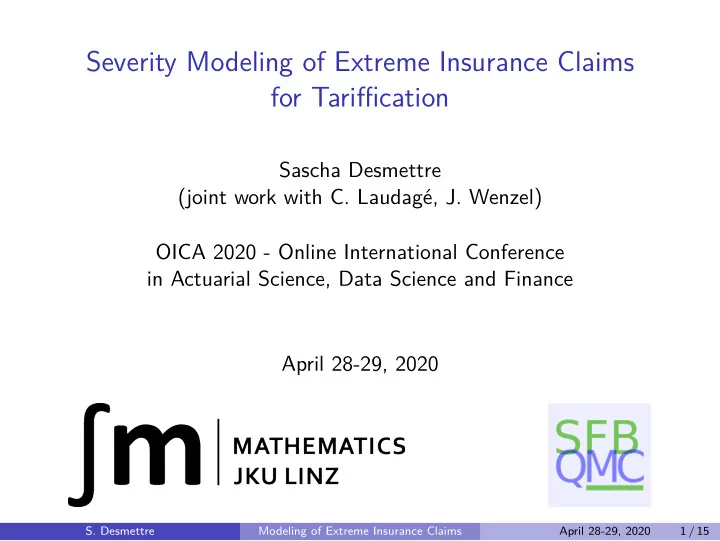
Severity Modeling of Extreme Insurance Claims for Tariffication

Sascha Desmettre (joint work with C. Laudagé, J. Wenzel) OICA 2020 - Online International Conference in Actuarial Science, Data Science and Finance April 28-29, 2020

• S. Desmettre

Modeling of Extreme Insurance Claims April 28-29, 2020 1 / 15

Motivation

Expected Claim Severity

◮ Usually modeled via generalized linear models (GLMs) based on gamma

distribution (see e.g. [Ohlsson & Johansson (10), Wüthrich (17)]).

Limitations

◮ Extreme claim sizes in data

The Gamma CDF is not heavy-tailed!

Concentration on body of distribution may lead to

◮ bias predictions ◮ missing robustness in predictions

Extreme Value Theory might help!

• S. Desmettre

Modeling of Extreme Insurance Claims April 28-29, 2020 2 / 15

Modeling Framework

Claim severity: Positive iid random RVs X1, X2, · · · ∼ X Claim frequency: Positive discrete RV N, where N ind. of X Features like car brand, age of driver or power of car affects damage. Vector of tariff features: R = (R1, . . . , Rd) with positive RVs Ri Tariff cell: Concrete combination of tariff features, e.g.

60 kW 80 kW . . . 18 years Cell 11 Cell 12 . . . 19 years Cell 21 Cell 22 . . . . . . . . . . . . ...

r = (19 years, 80 kW) What is the expected claim severity for a specific tariff cell r? E (X|R = r) Total damage in the given time period: E (S|R = r) = E (N|R = r) · E (X|R = r)

• S. Desmettre

Modeling of Extreme Insurance Claims April 28-29, 2020 3 / 15

Censoring by Insured Sum

Primary insurers only pay for damages up to a specified amount.

◮ Considered as tariff feature RI.

The actual damage Y may be larger than the insured sum. Claim severity is then given by X := min(Y , RI). Insurer only observes realizations for X, i.e. right-censored data. Determine the distribution of Y based on this censored data.

• S. Desmettre

Modeling of Extreme Insurance Claims April 28-29, 2020 4 / 15

Threshold Severity Model (TSM)

Split the distribution of Y at a certain threshold u > 0. Body and tail of the claim size distribution can be modeled separately. Notation for a given tariff cell r:

◮ Hr cdf for the body with parameter vector ΘH ◮ Gr cdf for the tail with parameter vector ΘG ◮ qr prob. of exceeding the given threshold u with parameter vector Θq

Assumptions to obtain a contiuous distribution function:

◮ Hr(u; ΘH) > 0 ◮ Gr(u; ΘG) = 0

• S. Desmettre

Modeling of Extreme Insurance Claims April 28-29, 2020 5 / 15

Concrete Specification of the TSM

Distribution function of Y with parameter vector Θ = (ΘH, ΘG, Θq): Fr (y; Θ) =

      

, y ≤ 0, (1 − qr (Θq)) Hr(y;ΘH)

Hr(u;ΘH)

, 0 < y ≤ u, (1 − qr (Θq)) + qr (Θq) Gr (y; ΘG) , y > u. Note: Threshold u independent of tariff cell r However, the exceeding probability depends on insured sum: qr (Θq) = 1 1 + e−(δ0+δI rI) with Θq = δ. ˆ Θ =

ˆ

ΘH, ˆ ΘG, ˆ Θq

• is estimated via maximizing the log-likelihood.

Obtain desired expectation for a tariff cell r by [X = min(Y , RI)]: Eˆ

Θ (min(Y , RI)|R = r) =

rI

yfr

• y; ˆ

Θ

• dy + rI
• 1 − Fr
• rI; ˆ

Θ

• .
• S. Desmettre

Modeling of Extreme Insurance Claims April 28-29, 2020 6 / 15

Recall: X := min(Y , RI).

• S. Desmettre

Modeling of Extreme Insurance Claims April 28-29, 2020 7 / 15

Estimators for Basic and Extreme Claim Sizes

Use concrete distributions for the conditional distribution functions below and above the threshold for a tariff cell r. Claim severity below the given threshold:

◮ Use general regression methods, i.e., a generalized linear model (GLM). ◮ Assume a gamma distribution for Hr. ◮ In particular, the conditional distribution function

P (Y ≤ y|Y ≤ u, R = r) = Hr (y; ΘH) Hr (u; ΘH), 0 < y ≤ u, describes a truncated gamma distribution.

Claim severity above the given threshold:

◮ Apply the peaks-over-threshold approach from extreme value theory. ◮ I.e., the conditional distribution function

P (Y ≤ y|Y > u, R = r) = Gr (y; ΘG) , y > u, is approximated by the generalized Pareto distribution (GPD).

• S. Desmettre

Modeling of Extreme Insurance Claims April 28-29, 2020 8 / 15

Basic Claim Sizes: Truncated Gamma GLM

We assume that for all covariates r ∈ Rd

≥0 we have

(Y |Y ≤ u, R = r) ∼ G (φ, θr, u) with φ > 0 , θr < 0 , i.e., they are truncated gamma distributed with dispersion φ, threshold u and scale θr, depending on the tariff features r. GLM to model conditional distribution function of X = min(Y , RI): P (X ≤ x|X ≤ u, R = r) = Hr (min(x, u); ΘH) Hr (u; ΘH) .

• θ (bu(.,ˆ

φ))

′

− − − − − − → E (X|X ≤ u, R = r)

g

− → α0 +

d

• i=1

ri αi, with (bu (θ, φ))

′ := b′ (θ) +

−u

• −θu

φ

1

φ −1 exp

• θu

φ

• γ
• 1

φ, −θu φ

• .
• S. Desmettre

Modeling of Extreme Insurance Claims April 28-29, 2020 9 / 15

Extreme Claim Sizes

We are looking at the excess distribution: Fu(y, r) = P (Y ≤ y|Y > u, R = r) = Gr (y; ΘG) , y > u. Theorem of Pickands, Balkema and de Haan: lim

u↑xF

sup

0<x<xF −u

• Fu (x) − Gξ,β(u) (x)
• = 0.

Application to Y with ΘG = (ξ, β) provides approximation : Gr (y; ΘG) = Gξ,β;u(y) = Gξ,β (y − u) , y > u. Conditional distribution function of X := min(Y , RI): P (X ≤ x|X > u, R = r) = Gξ,β (min (x, rI) − u) , x > u.

• S. Desmettre

Modeling of Extreme Insurance Claims April 28-29, 2020 10 / 15

Simulation Study

Goal: Show that the TSM outperforms the classical gamma GLM when fitting to simulated claim sizes from other regression models. Use heavy-tailed regression models based on the log-normal and Burr Type XII distributions to generate claim sizes. Present and compare the predictions stemming from the gamma GLM and the TSM w.r.t. the different scenarios. Setting:

◮ Set the index of the insured sum to 1 and denote it by v (= r1 = rI). ◮ Insured sums: 5 million, 20 million, 50 million. ◮ Second tariff feature taking integer values from 1 to 10.

[E.g. mileage or the car’s power; denoted by w (= r2)]. 30 tariff cells in total.

• S. Desmettre

Modeling of Extreme Insurance Claims April 28-29, 2020 11 / 15

Simulation Study: Log-Normal Regression

1 Simulate a normal random variable Z ∼ N (µ, σ) with mean

µ = α0 + α1 v + α1 w and standard deviation σ > 0.

2 Obtain the log-normal random variable by X = eZ. 3 In order to obtain a significant influence of the insured sum, we use

the following parameters in this scenario: α0 = 5.5, α1 = 4 × 10−8, α2 = 0.02, σ = 2.75.

4 Compare the classical gamma GLM with the TSM

in this log-normal setting.

• S. Desmettre

Modeling of Extreme Insurance Claims April 28-29, 2020 12 / 15

Simulation Study: Burr Regression

1 Simulate claim sizes from a Burr Type XII distribution, i.e,

Y ∼ Burr (β, λ, τ) with density fucntion fB (y; β, λ, τ) = λβλτyτ−1 (β + yτ)λ+1 , y > 0, β, λ, τ > 0.

2 To incorporate tariff cells, we use a regression for the parameter β,

i.e., we obtain the conditional distribution

(Y |R = r) ∼ Burr (β (r) , λ, τ) with β (r) := exp (τ (α0 + α1 v + α1 w)) .

3 Parameter values in this scenario:

α0 = 8, α1 = 4 × 10−8, α2 = 0.02, λ = 1.5, τ = 0.7 (⇒ heavy tails).

4 Compare the cl. gamma GLM with the TSM in this Burr-type setting.

• S. Desmettre

Modeling of Extreme Insurance Claims April 28-29, 2020 13 / 15

Results - Observed Statistics

Quantify the relative deviation between the true (µi) and predictive mean ( ˆ µi) of a specific tariff cell. Calculate (weighted) averages of the relative differences for every scenario w.r.t. all tariff cells: ¯ z1 := 1 30

30

• i=1

|ˆ µi − µi| µi , ¯ z2 :=

30

• i=1

mi m |ˆ µi − µi| µi . Simulated Claims Model ¯ z1 ¯ z2 Log-Normal Gamma GLM 53.31% 14.58% Log-Normal TSM 21.67% 13.35% Burr Gamma GLM 74.82% 23.51% Burr TSM 17.78% 5.59%

• S. Desmettre

Modeling of Extreme Insurance Claims April 28-29, 2020 14 / 15

Conclusion and Outlook

TSM combines idea of GLMs with EVT for tariffication. Allows for simple interpretations. Robust against Log-Normal and Burr claim sizes. Outperforms the classical gamma-based GLM. Further tariff features for excess distribution. Usage of different thresholds. Transfer to risk management.

• S. Desmettre

Modeling of Extreme Insurance Claims April 28-29, 2020 15 / 15

Literature

• C. Laudagé, S. Desmettre & J. Wenzel. “Severity Modeling of Extreme

Insurance Claims for Tariffication”. Insurance: Mathematics and Economics. 88 (2019) 77–92.

• T. Reynkens, R. Verbelen, J. Beirlant & K. Antonio. “Modelling censored

losses using splicing: A global fit strategy with mixed Erlang and extreme value distributions”. In: Insurance: Mathematics and Economics. 77 (2017) 65-77.

• P. Shi. “Fat-tailed regression models”. In: Predictive Modeling Applications

in Actuarial Science. 1 (2014) 236-259.

• P. Shi, X. Feng & A. Ivantsova. “Dependent frequency–severity modeling of

insurance claims”. In: Insurance: Mathematics and Economics. 64 (2015) 417–428.

• S. Desmettre

Modeling of Extreme Insurance Claims April 28-29, 2020 16 / 15

Literature

• E. Ohlsson, B. Johansson. “Non-Life Insurance Pricing with Generlaized

Linear Models”. Springer. (2010)

• M. Wüthrich. “Non-Life Insurance: Mathematics & Statistics”. Lecture Notes

available at SSRN. (2017).

• J. Garrrido, C. Genest, J. Schulz. “Generalized linear models for dependent

frequency and severity of insurance claims”. In: Insurance: Mathematics and

• Economics. 70 (2016) 205-215.
• D. Lee, W.K. Li & T.S.T Wong. “Modeling insurance claims via a mixture

exponential model combined with peaks-over-threshold approach”. In: Insurance: Mathematics and Economics. 51 (2012) 538-550.

• S. Desmettre

Modeling of Extreme Insurance Claims April 28-29, 2020 17 / 15

Definition Gamma and Truncated Gamma Distribution

For parameters α, β > 0 and the parametrization φ = 1/α > 0 and θ = −β/α < 0, we call a RV X ∼ G (φ, θ) with DF, resp. CDF fG (x; φ, θ) := βα xα−1 e−βx Γ (α) , x ≥ 0, FG (x; φ, θ) := γ (α, βx) Γ (α) , x ≥ 0, gamma distributed with dispersion parameter φ and scale parameter θ. For a given threshold u ∈ R>0, a RV X ∼ G (φ, θ, u) with DF fTG (x; φ, θ, u) := fG (x; φ, θ) FG (u; φ, θ)1(0,u] (x) , x ≥ 0, is said to be truncated gamma distributed.

• S. Desmettre

Modeling of Extreme Insurance Claims April 28-29, 2020 18 / 15

Simulated Claims in the TSM

Histogram of simulated claims (left) and simulated claims (right). Used parameters: u = 106, ξ = 0.4, β = 2400000, φ = 0.5, α0 = 10, α1 = 0, α2 = 1/5.

• S. Desmettre

Modeling of Extreme Insurance Claims April 28-29, 2020 19 / 15

Short Repetition: Generalized Linear Models (GLMS)

For now, let X denote the size of a claim. Basic idea: Density of X belongs to the exponential dispersion family: fX (x; θ, φ) = exp

xθ − b (θ)

φ\ω + c(x, φ, ω)

• ,

where

◮ φ is the dispersion parameter ◮ θ is the scaling parameter, ◮ b(θ) is the cumulant function, ◮ ω is a weight for e.g. the duration of a contract, ◮ c(x, φ, ω) is a normalization constant for fX.

Special case gamma distribution: b(θ) = − log(−θ), i.e., fX (x; θ, φ) exp(c(x, φ, ω)) = exp

xθ + log(−θ)

φ\ω

• S. Desmettre

Modeling of Extreme Insurance Claims April 28-29, 2020 20 / 15

Short Repetition: Functionality of GLMs

Generalization of linear regression that allows for response variables that have error distribution models other than a normal distribution. With the derivative of the CF b′ and link function g it holds: θ b′ − → E (X|R = r)

g

− → α0 +

d

• i=1

ri αi Distributional behavior of the claim size X, which is parametrized by θ, is described by the estimated regressors αi of the covariates ri. Logarithmic link function [leeds to multiplicative structure of premia]:

◮ E (X|R = r) = g−1(α0 +

d

• i=1

ri αi) = exp(α0 +

d

• i=1

ri αi)

◮ θ = (b′)−1 (E (X|R = r)) = (b′)−1

• exp(α0 +

d

• i=1

ri αi)

• S. Desmettre

Modeling of Extreme Insurance Claims April 28-29, 2020 21 / 15

Definition Generalized Pareto Distribution

For shape parameter ξ ∈ R, threshold u ∈ R and scale parameter β ∈ R>0 we define the distribution function Gξ,β;u by Gξ,β;u (x) =

  

1 −

• 1 + ξ x−u

β

− 1

ξ

, ξ = 0, 1 − e− x−u

β

, ξ = 0, where x ≥ u if ξ ≥ 0 and x ∈

• u, u − β

ξ

• if ξ < 0.

Then Gξ,β;u is called a generalized Pareto distribution (GPD). We denote the density of a GPD by gξ,β;u and set Gξ,β := Gξ,β;0.

• S. Desmettre

Modeling of Extreme Insurance Claims April 28-29, 2020 22 / 15