Sequences Sequences and Difference Equations "Sequences" - - PowerPoint PPT Presentation

5mm.

Sequences and Difference Equations (Appendix A)

Hans Petter Langtangen Simula Research Laboratory University of Oslo, Dept. of Informatics

Sequences and Difference Equations (Appendix A) – p.1/??

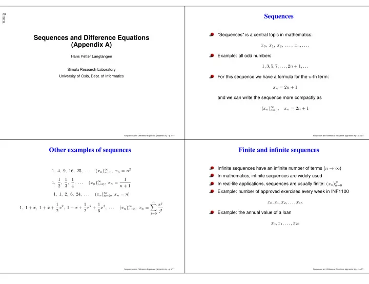
Sequences

"Sequences" is a central topic in mathematics: x0, x1, x2, . . . , xn, . . . , Example: all odd numbers 1, 3, 5, 7, . . . , 2n + 1, . . . For this sequence we have a formula for the n-th term: xn = 2n + 1 and we can write the sequence more compactly as (xn)∞

n=0,

xn = 2n + 1

Sequences and Difference Equations (Appendix A) – p.2/??

Other examples of sequences

1, 4, 9, 16, 25, . . . (xn)∞

n=0, xn = n2

1, 1 2, 1 3, 1 4, . . . (xn)∞

n=0, xn =

1 n + 1 1, 1, 2, 6, 24, . . . (xn)∞

n=0, xn = n!

1, 1 + x, 1 + x + 1 2x2, 1 + x + 1 2x2 + 1 6x3, . . . (xn)∞

n=0, xn = n

• j=0

xj j!

Sequences and Difference Equations (Appendix A) – p.3/??

Finite and infinite sequences

Infinite sequences have an infinite number of terms (n → ∞) In mathematics, infinite sequences are widely used In real-life applications, sequences are usually finite: (xn)N

n=0

Example: number of approved exercises every week in INF1100 x0, x1, x2, . . . , x15 Example: the annual value of a loan x0, x1, . . . , x20

Sequences and Difference Equations (Appendix A) – p.4/??

Difference equations

For sequences occuring in modeling of real-world phenomena, there is seldom a formula for the n-th term However, we can often set up one or more equations governing the sequence Such equations are called difference equations With a computer it is then very easy to generate the sequence by solving the difference equations Difference equations have lots of applications and are very easy to solve on a computer, but often complicated or impossible to solve for xn (as a formula) by pen and paper! The programs require only loops and arrays

Sequences and Difference Equations (Appendix A) – p.5/??

Modeling interest rates

Put x0 money in a bank at year 0. What is the value after N years if the interest rate is p percent per year? The fundamental information relates the value at year n, xn, to the value of the previous year, xn−1: xn = xn−1 + p 100xn−1 Solution by simulation: start with x0 (known) compute x1 = x0 + 0.01px0 = (1 + 0.01p)x0 compute x2 = x1 + 0.01px1 = (1 + 0.01p)2x0 ...continue this boring procedure... find that xn = (1 + 0.01p)nx0 ...which is what you learned in high school That is: we can solve this difference equation by hand

Sequences and Difference Equations (Appendix A) – p.6/??

Simulating the difference equation for interest rates

Simulate = solve math equations by repeating a simple procedure (relation) many times (boring, but well suited for a computer) Let us make a program for xn = xn−1 + p 100xn−1

from scitools.std import * x0 = 100 # initial amount p = 5 # interest rate N = 4 # number of years index_set = range(N+1) x = zeros(len(index_set)) # solution: x[0] = x0 for n in index_set[1:]: x[n] = x[n-1] + (p/100.0)*x[n-1] print x plot(index_set, x, ’ro’, xlabel=’years’, ylabel=’amount’)

Sequences and Difference Equations (Appendix A) – p.7/??

Note about the use of arrays

We store the xn values in a NumPy array To compute xn, we only need one previous value, xn−1 Thus, for the computations we do not need to store all the previous values, i.e., we do not need any array, just two numbers:

x_old = x0 for n in index_set[1:]: x_new = x_old + (p/100.)*x_old x_old = x_new # x_new becomes x_old at next step

However, programming with an array x[n] is simpler, safer, and enables plotting the sequence, so we will continue to use arrays in the examples

Sequences and Difference Equations (Appendix A) – p.8/??

Daily interest rate

A more relevant model is to add the interest every day The interest rate per day is r = p/D if p is the annual interest rate and D is the number of days in a year A common model in business applies D = 360, but n counts exact (all) days New model: xn = xn−1 + r 100xn−1 How can we find the number of days between two dates?

>>> import datetime >>> date1 = datetime.date(2007, 8, 3) # Aug 3, 2007 >>> date2 = datetime.date(2008, 8, 4) # Aug 4, 2008 >>> diff = date2 - date1 >>> print diff.days 367

Sequences and Difference Equations (Appendix A) – p.9/??

Program for daily interest rate

from scitools.std import * x0 = 100 # initial amount p = 5 # annual interest rate r = p/360.0 # daily interest rate import datetime date1 = datetime.date(2007, 8, 3) date2 = datetime.date(2011, 8, 3) diff = date2 - date1 N = diff.days index_set = range(N+1) x = zeros(len(index_set)) # solution: x[0] = x0 for n in index_set[1:]: x[n] = x[n-1] + (r/100.0)*x[n-1] print x plot(index_set, x, ’ro’, xlabel=’days’, ylabel=’amount’)

Sequences and Difference Equations (Appendix A) – p.10/??

But the annual interest rate may change quite often...

This is problematic when computing by hand In the program, a varying p is easy to deal with Just fill an array p with correct annual interest rate for day no. n,

n=0,...,N (this can be a bit challenging)

Modified program:

p = zeros(len(index_set)) # fill p[n] for n in index_set r = p/360.0 # daily interest rate x = zeros(len(index_set)) x[0] = x0 for n in index_set[1:]: x[n] = x[n-1] + (r[n-1]/100.0)*x[n-1]

Sequences and Difference Equations (Appendix A) – p.11/??

Payback of a loan

A loan L is paid back with a fixed amount L/N every month over N months + the interest rate of the loan Let p be the annual interest rate and p/12 the monthly rate Let xn be the value of the loan at the end of month n The fundamental relation from one month to the other: xn = xn−1 + p 12 · 100xn−1 − ( p 12 · 100xn−1 + L N ) which simplifies to xn = xn−1 − L N (The constant term L/N makes the equation nonhomogeneous, while the previous interest rate equation was homogeneous (all terms contain xn or xn−1)) The program is left as an exercise

Sequences and Difference Equations (Appendix A) – p.12/??

How to make a living from a fortune (part 1)

We have a fortune F invested with an annual interest rate of p percent Every year we plan to consume an amount cn (n counts years) Let xn be the development of our fortune A fundamental relation from one year to the other is xn = xn−1 + p 100xn−1 − cn Simplest possibility: keep cn constant Drawback: inflation demands cn to increase...

Sequences and Difference Equations (Appendix A) – p.13/??

How to make a living from a fortune (part 2)

Assume I percent inflation per year and that c0 is q percent of the interest the first year cn then develops as money with interest rate I, and xn develops with rate p but with a loss cn every year: xn = xn−1 + p 100xn−1 − cn−1, x0 = F, c0 = pq 104 F cn = cn−1 + I 100cn−1 This is a coupled system of two difference equations The programming is still simple: we update two arrays (x[n],

c[n]) inside the loop

Sequences and Difference Equations (Appendix A) – p.14/??

Fibonacci numbers; mathematics

No programming or math course is complete without an example

• n Fibonacci numbers!

Fibonacci derived the sequence by modeling rat populations, but the sequence of numbers has a range of peculiar mathematical properties and has therefore attracted much attention from mathematicians The difference equation reads xn = xn−1 + xn−2, x0 = 1, x1 = 1 This is a homogeneous difference equation of second order (three levels: n, n − 1, n − 2) – this classification is important for mathematical solution technique, but not for simulation in a program

Sequences and Difference Equations (Appendix A) – p.15/??

Fibonacci numbers; program

Program:

N = int(sys.argv[1]) from numpy import zeros x = zeros(N+1, int) x[0] = 1 x[1] = 1 for n in range(2, N+1): x[n] = x[n-1] + x[n-2] print n, x[n]

Sequences and Difference Equations (Appendix A) – p.16/??

Fibonacci numbers and overflow (part 1)

Run the program with N = 50:

2 2 3 3 4 5 5 8 6 13 ... 45 1836311903 Warning: overflow encountered in long_scalars 46 -1323752223

Can change int to long or int64 for array elements - now we can generate numbers up to N = 91 before we get overflow and garbage Can use float96 despite the fact that xn are integers (float gives only approximatively correct numbers) – now N up to 23600 is possible

Sequences and Difference Equations (Appendix A) – p.17/??

Fibonacci numbers and overflow (part 2)

Best: use Python scalars of type int – these automatically changes to long when overflow in int The long type in Python has arbitrarily many digits (as many as required in a computation) Note: long for arrays is 64 bit integer (int64), while scalar

long in Python is an integer with as "infinitely" many digits

Sequences and Difference Equations (Appendix A) – p.18/??

Program with Python’s long type for integers

The program now avoids arrays and makes use of three int

• bjects (which automatically changes to long when needed):

import sys N = int(sys.argv[1]) xnm1 = 1 # "x_n minus 1" xnm2 = 1 # "x_n minus 2" n = 2 while n <= N: xn = xnm1 + xnm2 print ’x_%d = %d’ % (n, xn) xnm2 = xnm1 xnm1 = xn n += 1

Run with N = 200:

x_2 = 2 x_3 = 3 ... x_198 = 173402521172797813159685037284371942044301 x_199 = 280571172992510140037611932413038677189525 x_200 = 453973694165307953197296969697410619233826

Can simulate until the computer’s memory becomes too small to store all the digits...

Sequences and Difference Equations (Appendix A) – p.19/??

Exponential growth with limited resources

The model for growth of money in a bank has a solution of the type xn = x0Cn (= x0en ln C) This is exponential growth in time (n) Populations of humans, animals, and cells also exhibit the same type of growth as long as there are unlimited resources (space and food) The environment can only support a maximum number M of individuals How can we model this? We shall introduce a logistic model

Sequences and Difference Equations (Appendix A) – p.20/??

Modeling logistic growth

Initially, when there are enough resources, the growth is exponential: xn = xn−1 + r 100xn−1 The growth rate r must decay to zero as xn approaches M A very simple r(n) function with this behavior is r(n) = ̺

• 1 − xn

M

• Observe that r(n) ≈ ̺ for small n when xn << M, and r(n) → 0

as xn → M and n is big The model for limited growth, called logistic growth, is then xn = xn−1 + ̺ 100xn−1

• 1 − xn−1

M

• Sequences and Difference Equations (Appendix A) – p.21/??

The evolution of logistic growth

In a program it is easy to introduce logistic instead of exponential growth, just replace

x[n] = x[n-1] + p/100.0)*x[n-1]

by

x[n] = x[n-1] + (rho/100.0)*x[n-1]*(1 - x[n-1]/float(M))

100 150 200 250 300 350 400 450 500 50 100 150 200 no of individuals time units

Sequences and Difference Equations (Appendix A) – p.22/??

The factorial as a difference equation

The factorial n! is defined as n(n − 1)(n − 2) · · · 1 (0! = 1) The following difference equation has xn = n! as solution and can be used to compute the factorial: xn = nxn−1, x0 = 1

Sequences and Difference Equations (Appendix A) – p.23/??

Taylor series as difference equations

The Taylor series for ex reads ex =

∞

• n=0

xn n! We can formulate this series as two coupled difference equations (and solving these difference equations is (probably) the most efficient way to compute the Taylor series!): an = x nan−1, a0 = 1 en = en−1 + an, e0 = 1 See the book for how to solve the difference equations by hand and show that the solution is the Taylor series for ex

Sequences and Difference Equations (Appendix A) – p.24/??

Newton’s method for finding zeros

Newton’s method for solving f(x) = 0 reads xn = xn−1 − f(xn−1) f ′(xn−1), x0 given This is a (nonlinear!) difference equation As n → ∞, we hope that xn → xs, where xs solves f(xs) = 0 Now we will not simulate N steps, because we do not know how large N must be in order to have xn as close to the exact solution xs as we want The program is therefore a bit different: we simulate the difference equation as long as f(x) > ǫ, where ǫ is small However, Newton’s method may (easily) diverge, so to avoid simulating forever, we stop when n > N

Sequences and Difference Equations (Appendix A) – p.25/??

A program for Newton’s method

A simple program can be

def Newton(f, x, dfdx, epsilon=1.0E-7, N=100): n = 0 while abs(f(x)) > epsilon and n <= N: x = x - f(x)/dfdx(x) n += 1 return x, n, f(x)

Note: f(x) is evaluated twice in each pass of the loop – only one evaluation is strictly necessary (can store the value in a variable and reuse it) Note: f(x)/dfdx(x) can give integer division Note: it could be handy to have an option for storing the x and

f(x) values in each iteration (for plotting or printing a

convergence table)

Sequences and Difference Equations (Appendix A) – p.26/??

A better program for Newton’s method

Only one f(x) call in each iteration, optional storage of (x, f(x)) values during the iterations, and float division:

def Newton(f, x, dfdx, epsilon=1.0E-7, N=100, store=False): f_value = f(x) n = 0 if store: info = [(x, f_value)] while abs(f_value) > epsilon and n <= N: x = x - float(f_value)/dfdx(x) n += 1 f_value = f(x) if store: info.append((x, f_value)) if store: return x, info else: return x, n, f_value

Sequences and Difference Equations (Appendix A) – p.27/??

Application of Newton’s method

Example: solve e−0.1x2 sin( π

2 x) = 0

from math import sin, cos, exp, pi import sys def g(x): return exp(-0.1*x**2)*sin(pi/2*x) def dg(x): return -2*0.1*x*exp(-0.1*x**2)*sin(pi/2*x) + \ pi/2*exp(-0.1*x**2)*cos(pi/2*x) x0 = float(sys.argv[1]) x, info = Newton(g, x0, dg, store=True) print ’zero:’, x for i in range(len(info)): print ’Iteration %3d: f(%g)=%g’ % \ (i, info[i][0], info[i][1])

Sequences and Difference Equations (Appendix A) – p.28/??

Results from this test problem

Start value 1.7:

zero: 1.999999999768449 Iteration 0: f(1.7)=0.340044 Iteration 1: f(1.99215)=0.00828786 Iteration 2: f(1.99998)=2.53347e-05 Iteration 3: f(2)=2.43808e-10

This works fine! Start value 3:

zero: 42.49723316011362 Iteration 0: f(3)=-0.40657 Iteration 1: f(4.66667)=0.0981146 Iteration 2: f(42.4972)=-2.59037e-79

WHAT???? Lesson learned: Newton’s method may work fine or give wrong results! You need to understand the method to interpret the results!

Sequences and Difference Equations (Appendix A) – p.29/??

Programming with sound

Sound on a computer = sequence of numbers Example: A 440 Hz This tone is a sine wave with frequency 440 Hz: s(t) = A sin (2πft) , f = 440 On a computer we represent s(t) by a discrete set of points on the function curve (exactly as we do when we plot s(t)) How many points (samples) along the curve do we need to use? CD quality needs 44100 samples per second

Sequences and Difference Equations (Appendix A) – p.30/??

Making a sound file with single tone (part 1)

r: sampling rate (samples per second, default 44100) f: frequency of the tone m: duration of the tone (seconds) Sampled sine function for this tone: sn = A sin

• 2πf n

r

• ,

n = 0, 1, . . . , m · r Code (we use descriptive names: frequency=f, length=m,

amplitude=A, sample_rate=r):

import numpy def note(frequency, length, amplitude=1, sample_rate=44100): time_points = numpy.linspace(0, length, length*sample_rate) data = numpy.sin(2*numpy.pi*frequency*time_points) data = amplitude*data return data

Sequences and Difference Equations (Appendix A) – p.31/??

Making a sound file with single tone (part 2)

We have data as an array with float and unit amplitude Sound data in a file should have 2-byte integers (int16) as data elements and amplitudes up to 215 − 1 (max value for int16 data)

data = note(440, 2) data = data.astype(numpy.int16) max_amplitude = 2**15 - 1 data = max_amplitude*data import scitools.sound scitools.sound.write(data, ’Atone.wav’) scitools.sound.play(’Atone.wav’)

Sequences and Difference Equations (Appendix A) – p.32/??

Reading sound from file

Let us read a sound file and add echo Sound = array s[n] Echo means to add a delay of the sound

# echo: e[n] = beta*s[n] + (1-beta)*s[n-b] def add_echo(data, beta=0.8, delay=0.002, sample_rate=44100): newdata = data.copy() shift = int(delay*sample_rate) # b (math symbol) for i in xrange(shift, len(data)): newdata[i] = beta*data[i] + (1-beta)*data[i-shift] return newdata

Load data, add echo and play:

data = scitools.sound.read(filename) data = data.astype(float) data = add_echo(data, beta=0.6) data = data.astype(int16) scitools.sound.play(data)

Sequences and Difference Equations (Appendix A) – p.33/??

Playing many notes

Each note is an array of samples from a sine with a frequency corresponding to the note Assume we have several note arrays data1, data2, ...:

# put data1, data2, ... after each other in a new array: data = numpy.concatenate((data1, data2, data3, ...))

The start of "Nothing Else Matters" (Metallica):

E1 = note(164.81, .5) G = note(392, .5) B = note(493.88, .5) E2 = note(659.26, .5) intro = numpy.concatenate((E1, G, B, E2, B, G)) ... song = numpy.concatenate((intro, intro, ...)) scitools.sound.play(song) scitools.sound.write(song, ’tmp.wav’)

Sequences and Difference Equations (Appendix A) – p.34/??

Summary of difference equations

Sequence: x0, x1, x2, . . ., xn, . . ., xN Difference equation: relation between xn, xn−1 and maybe xn−2 (or more terms in the "past") + known start value x0 (and more values x1, ... if more levels enter the equation) Solution of difference equations by simulation:

index_set = <array of n-values: 0, 1, ..., N> x = zeros(N+1) x[0] = x0 for n in index_set[1:]: x[n] = <formula involving x[n-1]>

Can have (simple) systems of difference equations:

for n in index_set[1:]: x[n] = <formula involving x[n-1]> y[n] = <formula involving y[n-1] and x[n]>

Taylor series and numerical methods such as Newton’s method can be formulated as difference equations, often resulting in a good way of programming the formulas

Sequences and Difference Equations (Appendix A) – p.35/??

Summarizing example: music of sequences

Given a x0, x1, x2, . . ., xn, . . ., xN Can we listen to this sequence as "music"? Yes, we just transform the xn values to suitable frequencies and use the functions in scitools.sound to generate tones We will study two sequences: xn = e−4n/N sin(8πn/N) and xn = xn−1 + qxn−1 (1 − xn−1) , x = x0 The first has values in [−1, 1], the other from x0 = 0.01 up to around 1 Transformation from "unit" xn to frequencies: yn = 440 + 200xn (first sequence then gives tones between 240 Hz and 640 Hz) Three functions: two for generating sequences, one for the sound

Sequences and Difference Equations (Appendix A) – p.36/??

Module file: soundeq.py

Look at files/soundeq.py for complete code. Try it out in these examples:

Unix/DOS> python soundseq.py oscillations 40 Unix/DOS> python soundseq.py logistic 100

Try to change the frequency range from 200 to 400.

Sequences and Difference Equations (Appendix A) – p.37/??