Sequences Sequences and Difference Equations "Sequences" - PDF document

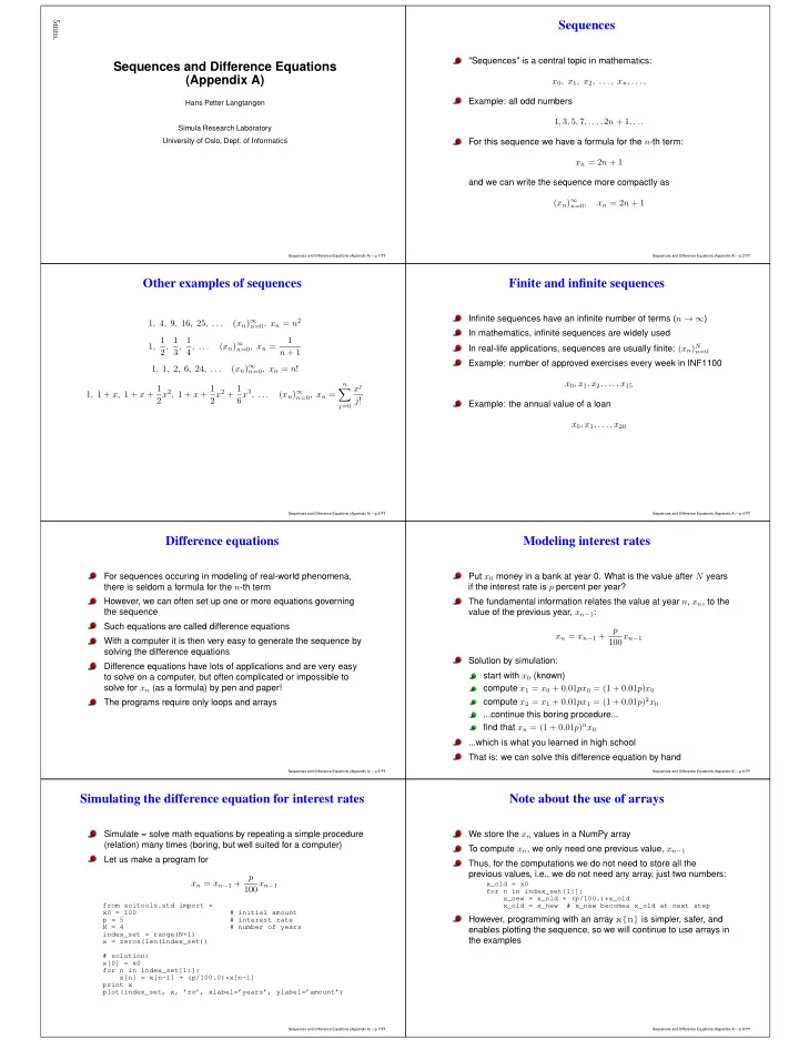
5mm. Sequences Sequences and Difference Equations "Sequences" is a central topic in mathematics: (Appendix A) x 0 , x 1 , x 2 , . . . , x n , . . . , Example: all odd numbers Hans Petter Langtangen 1 , 3 , 5 , 7 , . . . , 2 n + 1 , . . . Simula Research Laboratory University of Oslo, Dept. of Informatics For this sequence we have a formula for the n -th term: x n = 2 n + 1 and we can write the sequence more compactly as ( x n ) ∞ n =0 , x n = 2 n + 1 Sequences and Difference Equations (Appendix A) – p.1/ ?? Sequences and Difference Equations (Appendix A) – p.2/ ?? Other examples of sequences Finite and infinite sequences Infinite sequences have an infinite number of terms ( n → ∞ ) n =0 , x n = n 2 1 , 4 , 9 , 16 , 25 , . . . ( x n ) ∞ In mathematics, infinite sequences are widely used 1 , 1 2 , 1 3 , 1 1 ( x n ) ∞ 4 , . . . n =0 , x n = In real-life applications, sequences are usually finite: ( x n ) N n + 1 n =0 Example: number of approved exercises every week in INF1100 1 , 1 , 2 , 6 , 24 , . . . ( x n ) ∞ n =0 , x n = n ! x 0 , x 1 , x 2 , . . . , x 15 n 1 , 1 + x, 1 + x + 1 2 x 2 , 1 + x + 1 2 x 2 + 1 x j � 6 x 3 , . . . ( x n ) ∞ n =0 , x n = j ! Example: the annual value of a loan j =0 x 0 , x 1 , . . . , x 20 Sequences and Difference Equations (Appendix A) – p.3/ ?? Sequences and Difference Equations (Appendix A) – p.4/ ?? Difference equations Modeling interest rates For sequences occuring in modeling of real-world phenomena, Put x 0 money in a bank at year 0. What is the value after N years there is seldom a formula for the n -th term if the interest rate is p percent per year? However, we can often set up one or more equations governing The fundamental information relates the value at year n , x n , to the the sequence value of the previous year, x n − 1 : Such equations are called difference equations p x n = x n − 1 + 100 x n − 1 With a computer it is then very easy to generate the sequence by solving the difference equations Solution by simulation: Difference equations have lots of applications and are very easy start with x 0 (known) to solve on a computer, but often complicated or impossible to solve for x n (as a formula) by pen and paper! compute x 1 = x 0 + 0 . 01 px 0 = (1 + 0 . 01 p ) x 0 compute x 2 = x 1 + 0 . 01 px 1 = (1 + 0 . 01 p ) 2 x 0 The programs require only loops and arrays ...continue this boring procedure... find that x n = (1 + 0 . 01 p ) n x 0 ...which is what you learned in high school That is: we can solve this difference equation by hand Sequences and Difference Equations (Appendix A) – p.5/ ?? Sequences and Difference Equations (Appendix A) – p.6/ ?? Simulating the difference equation for interest rates Note about the use of arrays Simulate = solve math equations by repeating a simple procedure We store the x n values in a NumPy array (relation) many times (boring, but well suited for a computer) To compute x n , we only need one previous value, x n − 1 Let us make a program for Thus, for the computations we do not need to store all the previous values, i.e., we do not need any array, just two numbers: p x n = x n − 1 + 100 x n − 1 x_old = x0 for n in index_set[1:]: x_new = x_old + (p/100.)*x_old from scitools.std import * x_old = x_new # x_new becomes x_old at next step x0 = 100 # initial amount However, programming with an array x[n] is simpler, safer, and p = 5 # interest rate N = 4 # number of years enables plotting the sequence, so we will continue to use arrays in index_set = range(N+1) x = zeros(len(index_set)) the examples # solution: x[0] = x0 for n in index_set[1:]: x[n] = x[n-1] + (p/100.0)*x[n-1] print x plot(index_set, x, ’ro’, xlabel=’years’, ylabel=’amount’) Sequences and Difference Equations (Appendix A) – p.7/ ?? Sequences and Difference Equations (Appendix A) – p.8/ ??

Daily interest rate Program for daily interest rate from scitools.std import * A more relevant model is to add the interest every day x0 = 100 # initial amount p = 5 # annual interest rate The interest rate per day is r = p/D if p is the annual interest rate r = p/360.0 # daily interest rate and D is the number of days in a year import datetime date1 = datetime.date(2007, 8, 3) A common model in business applies D = 360 , but n counts exact date2 = datetime.date(2011, 8, 3) diff = date2 - date1 (all) days N = diff.days index_set = range(N+1) New model: x = zeros(len(index_set)) r x n = x n − 1 + 100 x n − 1 # solution: x[0] = x0 for n in index_set[1:]: How can we find the number of days between two dates? x[n] = x[n-1] + (r/100.0)*x[n-1] >>> import datetime print x >>> date1 = datetime.date(2007, 8, 3) # Aug 3, 2007 plot(index_set, x, ’ro’, xlabel=’days’, ylabel=’amount’) >>> date2 = datetime.date(2008, 8, 4) # Aug 4, 2008 >>> diff = date2 - date1 >>> print diff.days 367 Sequences and Difference Equations (Appendix A) – p.9/ ?? Sequences and Difference Equations (Appendix A) – p.10/ ?? But the annual interest rate may change quite often... Payback of a loan This is problematic when computing by hand A loan L is paid back with a fixed amount L/N every month over N months + the interest rate of the loan In the program, a varying p is easy to deal with Let p be the annual interest rate and p/ 12 the monthly rate Just fill an array p with correct annual interest rate for day no. n , n=0,...,N (this can be a bit challenging) Let x n be the value of the loan at the end of month n Modified program: The fundamental relation from one month to the other: p = zeros(len(index_set)) # fill p[n] for n in index_set p 12 · 100 x n − 1 + L p x n = x n − 1 + 12 · 100 x n − 1 − ( N ) r = p/360.0 # daily interest rate x = zeros(len(index_set)) which simplifies to x[0] = x0 for n in index_set[1:]: x n = x n − 1 − L x[n] = x[n-1] + (r[n-1]/100.0)*x[n-1] N (The constant term L/N makes the equation nonhomogeneous , while the previous interest rate equation was homogeneous (all terms contain x n or x n − 1 )) The program is left as an exercise Sequences and Difference Equations (Appendix A) – p.11/ ?? Sequences and Difference Equations (Appendix A) – p.12/ ?? How to make a living from a fortune (part 1) How to make a living from a fortune (part 2) We have a fortune F invested with an annual interest rate of p Assume I percent inflation per year and that c 0 is q percent of the percent interest the first year Every year we plan to consume an amount c n ( n counts years) c n then develops as money with interest rate I , and x n develops with rate p but with a loss c n every year: Let x n be the development of our fortune p x 0 = F, c 0 = pq A fundamental relation from one year to the other is x n = x n − 1 + 100 x n − 1 − c n − 1 , 10 4 F p I x n = x n − 1 + 100 x n − 1 − c n c n = c n − 1 + 100 c n − 1 Simplest possibility: keep c n constant This is a coupled system of two difference equations Drawback: inflation demands c n to increase... The programming is still simple: we update two arrays ( x[n] , c[n] ) inside the loop Sequences and Difference Equations (Appendix A) – p.13/ ?? Sequences and Difference Equations (Appendix A) – p.14/ ?? Fibonacci numbers; mathematics Fibonacci numbers; program No programming or math course is complete without an example Program: N = int(sys.argv[1]) on Fibonacci numbers! from numpy import zeros Fibonacci derived the sequence by modeling rat populations, but x = zeros(N+1, int) x[0] = 1 the sequence of numbers has a range of peculiar mathematical x[1] = 1 for n in range(2, N+1): properties and has therefore attracted much attention from x[n] = x[n-1] + x[n-2] mathematicians print n, x[n] The difference equation reads x n = x n − 1 + x n − 2 , x 0 = 1 , x 1 = 1 This is a homogeneous difference equation of second order (three levels: n , n − 1 , n − 2 ) – this classification is important for mathematical solution technique, but not for simulation in a program Sequences and Difference Equations (Appendix A) – p.15/ ?? Sequences and Difference Equations (Appendix A) – p.16/ ??