Sequence Based 100,071 genomes 96,985 pass quality checks - - PDF document

Sequence ¡Based ¡ Association ¡Studies

Gonçalo ¡Abecasis Center ¡for ¡Statistical ¡Genetics University ¡of ¡Michigan ¡School ¡of ¡Public ¡Health

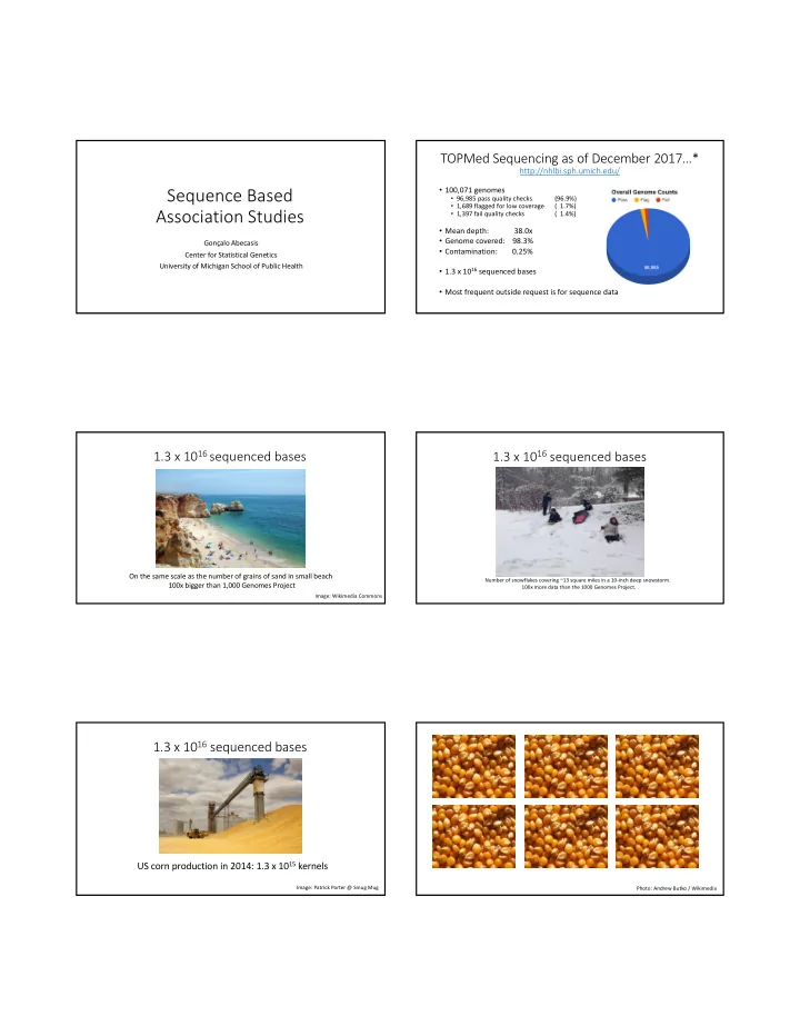
TOPMed ¡Sequencing ¡as ¡of ¡December ¡2017…* ¡

http://nhlbi.sph.umich.edu/

• 100,071 ¡genomes
• 96,985 ¡pass ¡quality ¡checks

(96.9%)

• 1,689 ¡flagged ¡for ¡low ¡coverage

( ¡ ¡1.7%)

• 1,397 ¡fail ¡quality ¡checks

( ¡ ¡1.4%)

• Mean ¡depth:

38.0x

• Genome ¡covered:

98.3%

• Contamination:

0.25%

• 1.3 ¡x ¡1016 sequenced ¡bases
• Most ¡frequent ¡outside ¡request ¡is ¡for ¡sequence ¡data

1.3 ¡x ¡1016 ¡sequenced ¡bases

On ¡the ¡same ¡scale ¡as ¡the ¡number ¡of ¡grains ¡of ¡sand ¡in ¡small ¡beach 100x ¡bigger ¡than ¡1,000 ¡Genomes ¡Project

Image: ¡Wikimedia ¡Commons

1.3 ¡x ¡1016 sequenced ¡bases

Number ¡of ¡snowflakes ¡covering ¡~13 ¡square ¡miles ¡in ¡a ¡10-­‑inch ¡deep ¡snowstorm. 100x ¡more ¡data ¡than ¡the ¡1000 ¡Genomes ¡Project.

1.3 ¡x ¡1016 sequenced ¡bases

US ¡corn ¡production ¡in ¡2014: ¡1.3 ¡x ¡1015 kernels

Image: ¡Patrick ¡Porter ¡@ ¡Smug ¡Mug Photo: ¡Andrew ¡Butko / ¡Wikimedia

Imagine, ¡two ¡cooks ¡and ¡one ¡corn ¡bread ¡recipe…

Images: ¡Wikimedia ¡Commons

Comparison ¡of ¡Raw ¡Calls

• 5 ¡samples ¡processed ¡in ¡duplicate ¡across ¡centers
• Raw ¡discrepancy ¡in ¡variant ¡calls
• 0.69% ¡-­‑ 2.93% ¡per ¡non-­‑reference ¡genotype
• Raw ¡discrepancy ¡after ¡harmonization
• 0.29% ¡– 0.48% ¡per ¡non-­‑reference ¡genotype
• Lower ¡if ¡we ¡filter ¡individual ¡calls ¡on ¡genotype ¡quality ¡or ¡depth

Study ¡1 Study ¡2 Study ¡3 Michigan ¡IRC

Sequence ¡QC ¡/ ¡Joint ¡Calling ¡/ ¡Harmonization

Sequencing ¡ Center Sequencing ¡ Center Study ¡4 Study ¡5 Study ¡6 University ¡of ¡Washington ¡DCC

Coordination ¡/ ¡Phenotype ¡Harmonization ¡/ ¡Analysis

NIH ¡NCBI

dbGAP // ¡Exchange ¡Area ¡// ¡SRA Long-­‑term ¡data ¡repository

TOPMed ¡Freeze ¡5: ¡Executive ¡Summary

• 64,960 ¡samples ¡and ¡470M ¡SNPs ¡and ¡indels
• First ¡freeze ¡where ¡bulk ¡of ¡computation ¡was ¡carried ¡out ¡on ¡commercial ¡clouds
• First ¡freeze ¡based ¡on ¡harmonized ¡data ¡processing ¡pipeline ¡developed ¡in ¡collaboration ¡with ¡CCDG
• The ¡Freeze ¡is ¡available ¡to ¡TOPMed ¡investigators ¡at:
• dbGap Exchange ¡Area ¡for ¡download ¡of ¡genotype ¡data
• https://encore.sph.umich.edu for ¡simple ¡association ¡analyses
• https://imputationserver.sph.umich.edu/ for ¡imputation ¡analyses ¡
• The ¡Freeze ¡is ¡available ¡to ¡everyone ¡at:
• https://bravo.sph.umich.edu for ¡browsing ¡variant ¡lists ¡only
• The ¡Freeze ¡is ¡the ¡largest ¡human ¡genome ¡variation ¡callset ¡known ¡to ¡us.
• The ¡Freeze ¡is ¡our ¡first ¡hg38 ¡callset. ¡
• The ¡Freeze ¡can ¡surely ¡be ¡improved. ¡If ¡you ¡see ¡something, ¡say ¡something.

471 ¡ 471 ¡million ¡ ¡variants, ¡ ¡217 ¡ 217 ¡million ¡ ¡singletons

Variant ¡Type Category # ¡PASS # ¡FAIL % dbSNP (PASS) Known/Novel Ts/Tv (PASS) SNP All 438M 85M 22.9% 1.93 / ¡1.69 Singleton 202M 24M 8.5% 1.23 ¡/ ¡1.54 Doubleton 69M 8.8M 12.6% 1.61 ¡/ ¡1.74 Tripleton ~ ¡0.1% 142M 24M 34.9% 2.23 ¡/ ¡1.99 0.1% ¡~ ¡1% 13M 4.5M 98.2% 2.17 ¡/ ¡1.79 1 ~ ¡10% 6.5M 2.9M 99.6% 1.82 ¡/ ¡1.75 >10% 5.3M 2.0M 99.8% 2.11 ¡/ ¡1.88 Indels All 33.4M 26.2M 20.1% Singleton 15.7M 4.7M 10.1% Doubleton 5.3M 1.8M 12.6% Tripleton ~ ¡0.1% 10.7M 8.0M 26.7% 0.1% ¡~ ¡1% 2.8M 968K 88.9% 1 ~ ¡10% 432K 2.3M 98.5% >10% 298K 1.4M 99.6%

Va Variant ¡ ¡Count Pe Per ¡ ¡Individual

Type SNPs Indels Average 3.48M 192K STDEV 301K 20.2K Max 4.07M 233K Min 3.01M 163K 25%-­‑ile 3.27M 177K Median 3.29M 179K 75%-­‑ile 3.88M 218K

Reassuringly, ¡SNP ¡and ¡indel ¡ counts ¡are ¡strongly ¡correlated

Si Sing ngleton ¡ n ¡Co Count Pe Per ¡ ¡Individual

Type SNPs Indels Average 3,019 235 STDEV 2,077 160 Max 41,110 3,141 Min 25%-­‑ile 1,591 124 Median 2,995 231 75%-­‑ile 3,948 311

Reassuringly, ¡SNP ¡and ¡indel ¡singleton ¡ counts ¡are ¡also ¡strongly ¡correlated

Ra Raw ¡ ¡“De ¡ ¡No Novo” ¡ ¡/ ¡ ¡Error ¡ ¡Ra Rate (Freeze ¡4)

~5,700 ¡singleton ¡SNPs ¡per ¡sample 1.3% ¡of ¡these ¡are ¡Mendelian ¡inconsistent ~300 ¡singleton ¡indels ¡per ¡sample 1.7% ¡of ¡these ¡are ¡Mendelian ¡inconsistent Browse ¡All ¡Variations ¡Online http://bravo.sph.umich.edu

KMT2D PCSK9

496 ¡missense, ¡26 ¡inframe indels, ¡0 ¡stop ¡or ¡frameshifts 91 ¡missense, ¡4 ¡inframe indels, ¡7 ¡stop ¡or ¡frameshifts Peter ¡VandeHaar

How ¡to ¡help ¡TOPMed advance ¡discoveries?

• Genomewide ¡analyses ¡at ¡scale ¡

are ¡challenging

• Even ¡simple ¡analysis ¡can ¡require ¡

1,000s ¡of ¡CPU ¡days ¡to ¡complete

• Need ¡to ¡engage ¡diverse ¡teams ¡in ¡

analysis ¡and ¡interpretation

snp,pvalue rs1234,0.05 rs4343,0.0002 rs51101,0.61 rs981,0.000018 rs2223,0.72

How ¡ENCORE ¡works ¡…

Matthew Flickinger Jonathon LeFaive

LDL ¡Genomewide ¡Analysis ¡in ¡ENCORE

Browsing ¡Variant ¡Lists ¡ Through ¡BRAVO

Peter ¡VandeHaar, ¡Daniel ¡Taliun

TOPMed ¡Variant ¡Browser

• TOPMed ¡Variants ¡Available ¡for ¡Browsing ¡at
• https://bravo.sph.umich.edu
• This ¡includes ¡a ¡subset ¡of ¡the ¡TOPMed ¡variants ¡from:
• Studies ¡and ¡individuals ¡from ¡whom ¡we ¡received ¡explicit ¡permission ¡to ¡

share ¡variant ¡list ¡in ¡BRAVO ¡and ¡submit ¡variants ¡to ¡dbSNP (rs#)

• The ¡VCF ¡file ¡corresponding ¡to ¡our ¡dbSNP submission ¡is ¡available ¡from ¡BRAVO ¡now ¡and ¡will ¡be ¡

available ¡from ¡dbSNP later ¡(as ¡customary).

• Accessing ¡BRAVO ¡requires ¡users ¡to ¡click-­‑through ¡terms ¡developed ¡in ¡collaboration ¡with ¡ELSI ¡

committee.

• Currently, ¡supporting ¡>1,000 ¡users ¡who ¡agreed ¡to ¡click-­‑through ¡terms ¡
• >100 ¡downloaded ¡dbSNP submission

ExAc Variant ¡Browser ¡(Daniel ¡MacArthur ¡et ¡al.) Current ¡State ¡of ¡Genetic ¡Association ¡Studies

• Surveying ¡common ¡variation ¡across ¡10,000s ¡-­‑ 100,000s ¡of ¡individuals ¡

is ¡now ¡routine

• Many ¡common ¡alleles ¡have ¡been ¡associated ¡with ¡a ¡variety ¡of ¡human ¡

complex ¡traits

• The ¡functional ¡consequences ¡of ¡these ¡alleles ¡are ¡often ¡subtle, ¡and ¡

translating ¡the ¡results ¡into ¡mechanistic ¡insights ¡remains ¡challenging

Goals ¡for ¡Sequence-­‑based ¡Studies

COMPLETE ¡GENETIC ¡ARCHITECTURE ¡OF ¡EACH ¡TRAIT

All ¡associated ¡risk ¡variants, ¡common, ¡rare, ¡SNPs, ¡indels ¡& ¡beyond

UNDERSTAND ¡FUNCTION ¡ LINKING ¡EACH ¡LOCUS ¡TO ¡DISEASE What ¡happens ¡in ¡gene ¡knockouts?

Use ¡sequencing ¡to ¡find ¡rare ¡human ¡“knockout” ¡alleles Why? ¡Results ¡of ¡animal ¡studies ¡and ¡in ¡vitro studies ¡often ¡murky

Next ¡Generation ¡Sequencing

Massive ¡Throughput ¡Sequencing

• Tools ¡to ¡generate ¡sequence ¡data ¡evolving ¡rapidly
• Commercial ¡platforms ¡now ¡produce ¡100s ¡of ¡gigabases of ¡sequence ¡

rapidly ¡and ¡at ¡low ¡cost ¡per ¡base

• Data ¡typically ¡consist ¡of ¡billions ¡of ¡short ¡sequence ¡reads ¡with ¡

moderate ¡accuracy

• 0.5 ¡– 1.0% ¡error ¡rates ¡per ¡base ¡are ¡typical

Shotgun ¡Sequence ¡Reads

• Typical ¡short ¡read ¡might ¡be ¡<25-­‑100 ¡bp long ¡and ¡not ¡

very ¡informative ¡on ¡its ¡own

• Reads ¡must ¡be ¡arranged ¡(aligned) relative ¡to ¡each ¡
• ther ¡to ¡reconstruct ¡longer ¡sequences

Read ¡Alignment

• The ¡first ¡step ¡in ¡analysis ¡of ¡human ¡short ¡read ¡data ¡is ¡to ¡align ¡each ¡read ¡to ¡

genome, ¡typically ¡using ¡a ¡hash ¡table ¡based ¡indexing ¡procedure

• This ¡process ¡now ¡takes ¡no ¡more ¡than ¡a ¡few ¡hours ¡per ¡10 ¡million ¡reads ¡…
• Analyzing ¡these ¡data ¡without ¡a ¡reference ¡human ¡genome ¡would ¡require ¡

much ¡longer ¡reads ¡or ¡result ¡in ¡very ¡fragmented ¡assemblies

5’-­‑ACTGGTCGATGCTAGCTGATAGCTAGCTAGCTGATGAGCCCGATCGCTGCTAGCTCGACG-­‑3’ Reference ¡Genome ¡(3,000,000,000 ¡bp) GCTAGCTGATAGCTAGCTAGCTGATGAGCCCGA Short ¡Read ¡(30-­‑100 ¡bp)

Read ¡Alignment ¡– Food ¡for ¡Thought

• Typically, ¡all ¡the ¡words ¡present ¡in ¡the ¡genome ¡are ¡indexed ¡to ¡facilitate ¡

read ¡mapping ¡…

• What ¡are ¡the ¡benefits ¡of ¡using ¡short ¡words?
• What ¡are ¡the ¡benefits ¡of ¡using ¡long ¡words?
• How ¡matches ¡do ¡you ¡expect, ¡on ¡average, ¡for ¡a ¡10-­‑base ¡word?
• Do ¡you ¡expect ¡large ¡deviations ¡from ¡this ¡average?

Calling ¡Consensus ¡Genotype ¡-­‑ Details

• Each ¡aligned ¡read ¡provides ¡a ¡small ¡amount ¡of ¡evidence ¡about ¡the ¡

underlying ¡genotype

• Read ¡may ¡be ¡consistent ¡with ¡a ¡particular ¡genotype ¡…
• Read ¡may ¡be ¡less ¡consistent ¡with ¡other ¡genotypes ¡…
• A ¡single ¡read ¡is ¡never ¡definitive
• This ¡evidence ¡is ¡cumulated ¡gradually, ¡until ¡we ¡reach ¡a ¡point ¡where ¡

the ¡genotype ¡can ¡be ¡called ¡confidently

• Let’s ¡outline ¡a ¡simple ¡approach ¡…

Shotgun ¡Sequence ¡Data

5’-­‑ACTGGTCGATGCTAGCTGATAGCTAGCTAGCTGATGAGCCCGATCGCTGCTAGCTCGACG-­‑3’ Reference ¡Genome GCTAGCTGATAGCTAGCTAGCTGATGAGCCCGA AGCTGATAGCTAGCTAGCTGATGAGCCCGATCGCTG ATGCTAGCTGATAGCTAGCTAGCTGATGAGCC ATAGCTAGATAGCTGATGAGCCCGATCGCTGCTAGCTC TAGCTGATAGCTAGATAGCTGATGAGCCCGAT Sequence ¡Reads Predicted ¡Genotype A/C

Shotgun ¡Sequence ¡Data

5’-­‑ACTGGTCGATGCTAGCTGATAGCTAGCTAGCTGATGAGCCCGATCGCTGCTAGCTCGACG-­‑3’ Reference ¡Genome Sequence ¡Reads Possible ¡Genotypes P(reads|A/A, ¡read ¡mapped)= ¡1.0 P(reads|A/C, ¡read ¡mapped)= ¡1.0 P(reads|C/C, ¡read ¡mapped)= ¡1.0

Shotgun ¡Sequence ¡Data

5’-­‑ACTGGTCGATGCTAGCTGATAGCTAGCTAGCTGATGAGCCCGATCGCTGCTAGCTCGACG-­‑3’ Reference ¡Genome GCTAGCTGATAGCTAGCTAGCTGATGAGCCCGA Sequence ¡Reads Possible ¡Genotypes P(reads|A/A, ¡read ¡mapped)= ¡P(C ¡observed|A/A, ¡read ¡mapped) ¡ P(reads|A/C, ¡read ¡mapped)= ¡P(C ¡observed|A/C, ¡read ¡mapped) ¡ P(reads|C/C, ¡read ¡mapped)= ¡P(C ¡observed|C/C, ¡read ¡mapped) ¡

Shotgun ¡Sequence ¡Data

5’-­‑ACTGGTCGATGCTAGCTGATAGCTAGCTAGCTGATGAGCCCGATCGCTGCTAGCTCGACG-­‑3’ Reference ¡Genome GCTAGCTGATAGCTAGCTAGCTGATGAGCCCGA Sequence ¡Reads Possible ¡Genotypes P(reads|A/A, ¡read ¡mapped)= ¡0.01 P(reads|A/C, ¡read ¡mapped)= ¡0.50 P(reads|C/C, ¡read ¡mapped)= ¡0.99

Shotgun ¡Sequence ¡Data

5’-­‑ACTGGTCGATGCTAGCTGATAGCTAGCTAGCTGATGAGCCCGATCGCTGCTAGCTCGACG-­‑3’ Reference ¡Genome GCTAGCTGATAGCTAGCTAGCTGATGAGCCCGA AGCTGATAGCTAGCTAGCTGATGAGCCCGATCGCTG Sequence ¡Reads Possible ¡Genotypes P(reads|A/A, ¡read ¡mapped)= ¡0.0001 P(reads|A/C ¡, ¡read ¡mapped)= ¡0.25 P(reads|C/C ¡, ¡read ¡mapped)= ¡0.98

Shotgun ¡Sequence ¡Data

5’-­‑ACTGGTCGATGCTAGCTGATAGCTAGCTAGCTGATGAGCCCGATCGCTGCTAGCTCGACG-­‑3’ Reference ¡Genome GCTAGCTGATAGCTAGCTAGCTGATGAGCCCGA AGCTGATAGCTAGCTAGCTGATGAGCCCGATCGCTG ATGCTAGCTGATAGCTAGCTAGCTGATGAGCC Sequence ¡Reads Possible ¡Genotypes P(reads|A/A ¡, ¡read ¡mapped)= ¡0.000001 P(reads|A/C ¡, ¡read ¡mapped)= ¡0.125 P(reads|C/C ¡, ¡read ¡mapped)= ¡0.97

Shotgun ¡Sequence ¡Data

5’-­‑ACTGGTCGATGCTAGCTGATAGCTAGCTAGCTGATGAGCCCGATCGCTGCTAGCTCGACG-­‑3’ Reference ¡Genome GCTAGCTGATAGCTAGCTAGCTGATGAGCCCGA AGCTGATAGCTAGCTAGCTGATGAGCCCGATCGCTG ATGCTAGCTGATAGCTAGCTAGCTGATGAGCC ATAGCTAGATAGCTGATGAGCCCGATCGCTGCTAGCTC Sequence ¡Reads Possible ¡Genotypes P(reads|A/A ¡, ¡read ¡mapped)= ¡0.00000099 P(reads|A/C ¡, ¡read ¡mapped)= ¡0.0625 P(reads|C/C ¡, ¡read ¡mapped)= ¡0.0097

Shotgun ¡Sequence ¡Data

5’-­‑ACTGGTCGATGCTAGCTGATAGCTAGCTAGCTGATGAGCCCGATCGCTGCTAGCTCGACG-­‑3’ Reference ¡Genome GCTAGCTGATAGCTAGCTAGCTGATGAGCCCGA AGCTGATAGCTAGCTAGCTGATGAGCCCGATCGCTG ATGCTAGCTGATAGCTAGCTAGCTGATGAGCC ATAGCTAGATAGCTGATGAGCCCGATCGCTGCTAGCTC TAGCTGATAGCTAGATAGCTGATGAGCCCGAT Sequence ¡Reads Possible ¡Genotypes P(reads|A/A ¡, ¡read ¡mapped)= ¡0.00000098 P(reads|A/C ¡, ¡read ¡mapped)= ¡0.03125 P(reads|C/C ¡, ¡read ¡mapped)= ¡0.000097

Shotgun ¡Sequence ¡Data

5’-­‑ACTGGTCGATGCTAGCTGATAGCTAGCTAGCTGATGAGCCCGATCGCTGCTAGCTCGACG-­‑3’ Reference ¡Genome GCTAGCTGATAGCTAGCTAGCTGATGAGCCCGA AGCTGATAGCTAGCTAGCTGATGAGCCCGATCGCTG ATGCTAGCTGATAGCTAGCTAGCTGATGAGCC ATAGCTAGATAGCTGATGAGCCCGATCGCTGCTAGCTC TAGCTGATAGCTAGATAGCTGATGAGCCCGAT Sequence ¡Reads Combine ¡these ¡likelihoods ¡with ¡a ¡prior ¡incorporating ¡information ¡from ¡other ¡ individuals ¡and ¡flanking ¡sites ¡to ¡assign ¡a ¡genotype. P(reads|A/A, ¡read ¡mapped)= ¡0.00000098 P(reads|A/C, ¡read ¡mapped)= ¡0.03125 P(reads|C/C, ¡read ¡mapped)= ¡0.000097

From ¡Sequence ¡to ¡Genotype: Individual ¡Based ¡Prior

5’-­‑ACTGGTCGATGCTAGCTGATAGCTAGCTAGCTGATGAGCCCGATCGCTGCTAGCTCGACG-­‑3’ Reference ¡Genome GCTAGCTGATAGCTAGCTAGCTGATGAGCCCGA AGCTGATAGCTAGCTAGCTGATGAGCCCGATCGCTG ATGCTAGCTGATAGCTAGCTAGCTGATGAGCC ATAGCTAGATAGCTGATGAGCCCGATCGCTGCTAGCTC TAGCTGATAGCTAGATAGCTGATGAGCCCGAT Sequence ¡Reads Individual ¡Based ¡Prior: ¡Every ¡site ¡has ¡1/1000 ¡probability ¡of ¡varying. P(reads|A/A)= ¡0.00000098 Prior(A/A) ¡= ¡0.00034 Posterior(A/A) ¡= ¡<.001 P(reads|A/C)= ¡0.03125 Prior(A/C) ¡= ¡0.00066 Posterior(A/C) ¡= 0.175 P(reads|C/C)= ¡0.000097 Prior(C/C) ¡= ¡0.99900 Posterior(C/C) ¡= 0.825

From ¡Sequence ¡to ¡Genotype: Individual ¡Based ¡Prior

5’-­‑ACTGGTCGATGCTAGCTGATAGCTAGCTAGCTGATGAGCCCGATCGCTGCTAGCTCGACG-­‑3’ Reference ¡Genome GCTAGCTGATAGCTAGCTAGCTGATGAGCCCGA AGCTGATAGCTAGCTAGCTGATGAGCCCGATCGCTG ATGCTAGCTGATAGCTAGCTAGCTGATGAGCC ATAGCTAGATAGCTGATGAGCCCGATCGCTGCTAGCTC TAGCTGATAGCTAGATAGCTGATGAGCCCGAT Sequence ¡Reads Individual ¡Based ¡Prior: ¡Every ¡site ¡has ¡1/1000 ¡probability ¡of ¡varying. P(reads|A/A)= ¡0.00000098 Prior(A/A) ¡= ¡0.00034 Posterior(A/A) ¡= ¡<.001 P(reads|A/C)= ¡0.03125 Prior(A/C) ¡= ¡0.00066 Posterior(A/C) ¡= 0.175 P(reads|C/C)= ¡0.000097 Prior(C/C) ¡= ¡0.99900 Posterior(C/C) ¡= 0.825

Shotgun ¡Sequence ¡Data

Haplotype ¡Based ¡Prior

5’-­‑ACTGGTCGATGCTAGCTGATAGCTAGCTAGCTGATGAGCCCGATCGCTGCTAGCTCGACG-­‑3’ Reference ¡Genome GCTAGCTGATAGCTAGCTAGCTGATGAGCCCGA AGCTGATAGCTAGCTAGCTGATGAGCCCGATCGCTG ATGCTAGCTGATAGCTAGCTAGCTGATGAGCC ATAGCTAGATAGCTGATGAGCCCGATCGCTGCTAGCTC TAGCTGATAGCTAGATAGCTGATGAGCCCGAT Sequence ¡Reads Haplotype ¡Based ¡Prior: ¡Examine ¡other ¡chromosomes ¡that ¡are ¡similar ¡at ¡locus ¡of ¡interest. In ¡the ¡example ¡above, ¡we ¡estimated ¡that ¡20% ¡of ¡similar ¡chromosomes ¡carry ¡allele ¡A. P(reads|A/A)= ¡0.00000098 Prior(A/A) ¡= ¡0.04 Posterior(A/A) ¡= ¡<.001 P(reads|A/C)= ¡0.03125 Prior(A/C) ¡= ¡0.32 Posterior(A/C) ¡= 0.999 P(reads|C/C)= ¡0.000097 Prior(C/C) ¡= ¡0.64 Posterior(C/C) ¡= <.001

Shotgun ¡Sequence ¡Data

Haplotype ¡Based ¡Prior

5’-­‑ACTGGTCGATGCTAGCTGATAGCTAGCTAGCTGATGAGCCCGATCGCTGCTAGCTCGACG-­‑3’ Reference ¡Genome GCTAGCTGATAGCTAGCTAGCTGATGAGCCCGA AGCTGATAGCTAGCTAGCTGATGAGCCCGATCGCTG ATGCTAGCTGATAGCTAGCTAGCTGATGAGCC ATAGCTAGATAGCTGATGAGCCCGATCGCTGCTAGCTC TAGCTGATAGCTAGATAGCTGATGAGCCCGAT Sequence ¡Reads Haplotype ¡Based ¡Prior: ¡Examine ¡other ¡chromosomes ¡that ¡are ¡similar ¡at ¡locus ¡of ¡interest. In ¡the ¡example ¡above, ¡we ¡estimated ¡that ¡20% ¡of ¡similar ¡chromosomes ¡carry ¡allele ¡A. P(reads|A/A)= ¡0.00000098 Prior(A/A) ¡= ¡0.04 Posterior(A/A) ¡= ¡<.001 P(reads|A/C)= ¡0.03125 Prior(A/C) ¡= ¡0.32 Posterior(A/C) ¡= 0.999 P(reads|C/C)= ¡0.000097 Prior(C/C) ¡= ¡0.64 Posterior(C/C) ¡= <.001

Sequence ¡Based ¡Genotype ¡Calls

• Individual ¡Based ¡Prior
• Assumes ¡all ¡sites ¡have ¡an ¡equal ¡probability ¡of ¡showing ¡polymorphism
• Specifically, ¡assumption ¡is ¡that ¡about ¡1/1000 ¡bases ¡differ ¡from ¡reference
• If ¡reads ¡where ¡error ¡free ¡and ¡sampling ¡Poisson ¡…
• … ¡14x ¡coverage ¡would ¡allow ¡for ¡99.8% ¡genotype ¡accuracy
• … ¡30x ¡coverage ¡of ¡the ¡genome ¡needed ¡to ¡allow ¡for ¡errors ¡and ¡clustering
• Population ¡Based ¡Prior
• Uses ¡frequency ¡information ¡obtained ¡from ¡examining ¡other ¡individuals
• Calling ¡very ¡rare ¡polymorphisms ¡still ¡requires ¡20-­‑30x ¡coverage ¡of ¡the ¡genome
• Calling ¡common ¡polymorphisms ¡requires ¡much ¡less ¡data
• Haplotype ¡Based ¡Prior ¡or ¡Imputation ¡Based ¡Analysis
• Compares ¡individuals ¡with ¡similar ¡flanking ¡haplotypes
• Calling ¡very ¡rare ¡polymorphisms ¡still ¡requires ¡20-­‑30x ¡coverage ¡of ¡the ¡genome
• Can ¡make ¡accurate ¡genotype ¡calls ¡with ¡2-­‑4x ¡coverage ¡of ¡the ¡genome
• Accuracy ¡improves ¡as ¡more ¡individuals ¡are ¡sequenced

Low-­‑Pass ¡Sequencing: Sketch ¡of ¡Methodology

Re Recipe: ¡ ¡Genotypes ¡ ¡for ¡ ¡Shotgun ¡ ¡Sequence ¡ ¡Data

• Start ¡with ¡some ¡plausible ¡configuration ¡for ¡each ¡individual
• Use ¡Markov ¡model ¡to ¡update ¡one ¡individual ¡conditional ¡on ¡all ¡others
• Repeat ¡previous ¡step ¡many ¡times
• Generate ¡a ¡consensus ¡genotypes ¡and ¡haplotypes ¡for ¡each ¡individual

Silly ¡Cartoon ¡View ¡of ¡Shot ¡Gun ¡Data

. G . G A . . T . C . T . T . . . . T G . C . A . . . C T C C C . . . C . . . . . . C C A . G . . C T . . . . . . . . . T G . . . . . . . . C T T T . C . . . . . . . . . . . . . . T . . C . . A C C . . A T G . . . . . . . C . C C . G A C C . C A . G G C G A . A . . . . . . G . C . . T . T . . . . . . . . . C . T . T . . . . . . . A . C G . . A . . C T . . . . . C T . G . . . C G A A . . T . . T . T . T . C T . . G C . G A . A T C . . C . T . T T . . . . G . . . A . . . . . . C C . A C . T C A T G . . . A . G . . C . T T . . . T . T G . G C C G A . . . T . . T . . . T T . T . . G C . . . G A C . C . . . . . . . . . . T G . T . . . . T . . C . . . . C C . . . . . . . . . G A T C . C C . G . . C T T . . G C . . . G A . T . T T . T . T T . T . . . . . G A G . . T . T . . G A . . T C G . . C . . A A . . T . . . . . . . . . . . . G .

Silly ¡Cartoon ¡View ¡of ¡Shot ¡Gun ¡Data

c ¡ G ¡ a ¡ G ¡ A ¡ t ¡ c ¡ T ¡ c ¡ C ¡ t ¡ T ¡ c ¡ T ¡ t ¡ c ¡ t ¡ g ¡ T ¡ G ¡ c ¡ C ¡ g ¡ A ¡ g ¡ a ¡ t ¡ C ¡ T ¡ C ¡ C ¡ C ¡ g ¡ a ¡ c ¡ C ¡ t ¡ c ¡ a ¡ t ¡ g ¡ g ¡ C ¡ C ¡ A ¡ a ¡ G ¡ c ¡ t ¡ C ¡ T ¡ t ¡ t ¡ t ¡ c ¡ t ¡ t ¡ c ¡ t ¡ g ¡ T ¡ G ¡ c ¡ c ¡ g ¡ a ¡ a ¡ g ¡ c ¡ t ¡ C ¡ T ¡ T ¡ T ¡ t ¡ C ¡ t ¡ t ¡ c ¡ t ¡ g ¡ t ¡ g ¡ c ¡ c ¡ g ¡ a ¡ g ¡ a ¡ c ¡ T ¡ c ¡ t ¡ C ¡ c ¡ g ¡ A ¡ C ¡ C ¡ t ¡ t ¡ A ¡ T ¡ G ¡ c ¡ t ¡ g ¡ g ¡ g ¡ a ¡ t ¡ C ¡ t ¡ C ¡ C ¡ c ¡ G ¡ A ¡ C ¡ C ¡ t ¡ C ¡ A ¡ t ¡ G ¡ G ¡ C ¡ G ¡ A ¡ g ¡ A ¡ t ¡ c ¡ t ¡ c ¡ c ¡ c ¡ G ¡ a ¡ C ¡ c ¡ t ¡ T ¡ g ¡ T ¡ g ¡ c ¡ c ¡ g ¡ a ¡ g ¡ a ¡ c ¡ t ¡ C ¡ t ¡ T ¡ t ¡ T ¡ c ¡ t ¡ t ¡ t ¡ t ¡ g ¡ t ¡ A ¡ c ¡ C ¡ G ¡ a ¡ g ¡ A ¡ c ¡ t ¡ C ¡ T ¡ c ¡ c ¡ g ¡ a ¡ c ¡ C ¡ T ¡ c ¡ G ¡ t ¡ g ¡ c ¡ C ¡ G ¡ A ¡ A ¡ g ¡ c ¡ T ¡ c ¡ t ¡ T ¡ t ¡ T ¡ c ¡ T ¡ t ¡ C ¡ T ¡ g ¡ t ¡ G ¡ C ¡ c ¡ G ¡ A ¡ g ¡ A ¡ T ¡ C ¡ t ¡ c ¡ C ¡ t ¡ T ¡ c ¡ T ¡ T ¡ c ¡ t ¡ g ¡ t ¡ G ¡ c ¡ c ¡ g ¡ A ¡ g ¡ a ¡ t ¡ c ¡ t ¡ c ¡ C ¡ C ¡ g ¡ A ¡ C ¡ c ¡ T ¡ C ¡ A ¡ T ¡ G ¡ g ¡ c ¡ c ¡ A ¡ a ¡ G ¡ c ¡ t ¡ C ¡ t ¡ T ¡ T ¡ t ¡ c ¡ t ¡ T ¡ c ¡ T ¡ G ¡ t ¡ G ¡ C ¡ C ¡ G ¡ A ¡ a ¡ g ¡ c ¡ T ¡ c ¡ t ¡ T ¡ t ¡ t ¡ c ¡ T ¡ T ¡ c ¡ T ¡ g ¡ t ¡ G ¡ C ¡ c ¡ g ¡ a ¡ G ¡ A ¡ C ¡ t ¡ C ¡ t ¡ c ¡ c ¡ g ¡ a ¡ c ¡ c ¡ t ¡ t ¡ a ¡ T ¡ G ¡ c ¡ T ¡ g ¡ g ¡ g ¡ a ¡ T ¡ c ¡ t ¡ C ¡ c ¡ c ¡ g ¡ a ¡ C ¡ C ¡ t ¡ c ¡ a ¡ t ¡ g ¡ g ¡ c ¡ g ¡ a ¡ G ¡ A ¡ T ¡ C ¡ t ¡ C ¡ C ¡ c ¡ G ¡ a ¡ c ¡ C ¡ T ¡ T ¡ g ¡ t ¡ G ¡ C ¡ c ¡ g ¡ a ¡ G ¡ A ¡ c ¡ T ¡ c ¡ T ¡ T ¡ t ¡ T ¡ c ¡ T ¡ T ¡ t ¡ T ¡ g ¡ t ¡ a ¡ c ¡ c ¡ G ¡ A ¡ G ¡ a ¡ c ¡ T ¡ c ¡ T ¡ c ¡ c ¡ G ¡ A ¡ c ¡ c ¡ T ¡ C ¡ G ¡ t ¡ g ¡ C ¡ c ¡ g ¡ A ¡ A ¡ g ¡ c ¡ T ¡ c ¡ t ¡ t ¡ t ¡ t ¡ c ¡ t ¡ t ¡ c ¡ t ¡ g ¡ t ¡ G ¡ c ¡

How ¡to ¡Update ¡One ¡Pair ¡of ¡Haplotypes?

• Markov ¡model ¡similar ¡to ¡those ¡that ¡describe ¡haplotype ¡sharing
• To ¡carry ¡out ¡an ¡update, ¡select ¡one ¡individual
• Fix ¡(temporarily) ¡interim ¡haplotype ¡estimates ¡for ¡all ¡other ¡individuals
• Describe ¡selected ¡individual ¡as ¡mosaic ¡of ¡other ¡available ¡haplotypes
• Select ¡mosaic ¡pieces ¡that ¡fit ¡well ¡with ¡available ¡sequence ¡data

Markov ¡Model

1

X

2

X

3

X

M

X

2

S

3

S

M

S

1

S

) | (

1 2 S

S P ) | (

2 3 S

S P (...) P ) | (

1 1 S

X P ) | (

2 2 S

X P ) | (

3 3 S

X P ) | (

M M S

X P Model ¡is ¡very ¡similar ¡to ¡the ¡one ¡we ¡previously ¡used ¡for ¡imputatoin… ) (

1

S P

Likelihood

åå å Õ Õ

= =

• 

=

1 2

1 2 1 1

) | ( ) | ( ) ( ...

S S S M i i i M i i i

M

S X P S S P S P L

• P(S1) ¡= ¡1 ¡/ ¡H2 where ¡H ¡is ¡the ¡number ¡of ¡template ¡haplotypes
• P(Si|Si-­‑1) ¡depends ¡on ¡estimated ¡population ¡recombination ¡rate
• P(Xi|Si) ¡are ¡the ¡genotype ¡likelihoods

Ge Genotypes ¡ ¡with ¡ ¡Shotgun ¡ ¡Sequence ¡ ¡Data (Pr Predictions ¡ ¡as ¡ ¡of ¡ ¡2008)

• Sequence ¡400 ¡individuals ¡at ¡2x ¡depth
• Assume ¡error ¡rate ¡is ¡of ¡about ¡0.5%
• If ¡we ¡analyze ¡a ¡single ¡individual, ¡almost ¡impossible ¡to ¡call ¡genotypes
• False ¡positives ¡due ¡to ¡error, ¡1 ¡in ¡every ¡100 ¡bases
• Allele ¡of ¡interest ¡not ¡sampled, ¡1 ¡in ¡every ¡two ¡heterozygous ¡sites
• If ¡we ¡do ¡an ¡imputation ¡based ¡analysis
• Expect ¡to ¡call ¡genotypes ¡with ¡99.7% ¡accuracy ¡for ¡sites ¡with ¡frequency ¡>1%

Yun ¡Li

The ¡1000 ¡Genomes ¡Project 1000 ¡Genome ¡Project ¡Goals ¡(2008)

• >95% ¡of ¡accessible ¡genetic ¡variants

with ¡a ¡frequency ¡of ¡>1% ¡ in ¡each ¡of ¡multiple ¡continental ¡regions

• Define ¡haplotype ¡structure ¡in ¡the ¡genome
• Develop ¡methods ¡for ¡analysis ¡and ¡interpretation ¡of ¡sequence ¡data
• Project ¡set ¡out ¡to ¡achieve ¡these ¡using ¡low ¡coverage ¡sequencing

Samples ¡in ¡the ¡final ¡phase

ACB 96 ASW 61 BEB 86 CDX 93 CEU 99 CHB 103 CHS 105 CLM 94 ESN 99 FIN 99 GBR 90 GIH 103 GWD 113 IBS 107 ITU 102 JPT 104 KHV 99 LWK 99 MSL 85 MXL 64 PEL 85 PJL 96 PUR 104 STU 102 TSI 107 YRI 108

Variants ¡per ¡genome

3.8 4 4.2 4.4 4.6 4.8 5 5.2 MSL ESN YRI LWK GWD ACB ASW PUR CLM MXL PEL KHV CHB JPT CDX CHS BEB ITU STU GIH PJL TSI IBS CEU GBR FIN Individual Allele Count (Million)

Type Variant sites ¡/ ¡ genome SNPs ~3,800,000 Indels ~570,000 Mobile ¡Element ¡ Insertions ~1000 Large ¡Deletions ~1000 CNVs ~150 Inversions ~11

Population ¡histories

0.0 2.5 10 20 50 100 200 500 1000 2000 Thousands of Years (assuming g=25 yrs, μ=2.5x10-8 / bp / yr) Effective Population Size (x 104) ACB ASW CDX CHB CHS JPT KHV CLM MXL PEL PUR CEU FIN GBR IBS TSI BEB GIH ITU PJL STU ESN GWD LWK MSL YRI

CHB KHV ASW LWK MXL FIN CHS JPT TSI PJL STU ITU CDX CEU PUR IBS GIH GBR CLM MSL ACB GWD YRI ESN BEB PEL

Does ¡Haplotype ¡Information ¡Really ¡Help?

Genotype ¡Accuracy ¡for ¡4x ¡Sequence ¡Data

Haplotype ¡Aware ¡Priors Population-­‑Based ¡Priors

Hyun ¡Min ¡Kang, ¡1000 ¡Genomes ¡Project

Optimal ¡Model ¡for ¡Analyzing ¡1000 ¡Genomes?

1000 ¡Genomes ¡Call ¡Set (CEU) Homozygous Reference Error Heterozygote ¡Error Homozygous ¡Non-­‑ Reference ¡Error Broad 0.66 4.29 3.80 Michigan 0.68 3.26 3.06 Sanger 1.27 3.43 2.60

• Michigan ¡caller ¡combines ¡…

– Markov ¡models ¡to ¡identify ¡shared ¡haplotypes, – Classifiers ¡to ¡distinguish ¡true ¡variants ¡from ¡error, – Strategies ¡to ¡distribute ¡computation ¡across ¡cluster

Optimal ¡Model ¡for ¡Analyzing ¡1000 ¡Genomes?

1000 ¡Genomes ¡Call ¡Set (CEU) Homozygous Reference Error Heterozygote ¡Error Homozygous ¡Non-­‑ Reference ¡Error Broad 0.66 4.29 3.80 Michigan 0.68 3.26 3.06 Sanger 1.27 3.43 2.60 Majority Consensus 0.45 2.05 2.21

• Common ¡to ¡see ¡“ensemble” ¡methods ¡
• utperform ¡the ¡best ¡single ¡method

Current ¡1000 ¡Genomes ¡Analysis ¡Pipeline

10 ¡SNP/INDEL ¡callsets, 2 ¡STR ¡callsets, 12 ¡SV ¡callsets

Raw ¡ data 24 ¡initial ¡ callsets Consensus callsets Integration Final callset

Genotyping ¡ arrays Low ¡ Coverage ¡ and ¡Exome ¡ Read ¡Data Callset 1 Callset 2 Callset 3 Callset n Callset 4 Callset 5 SNPs ¡and ¡high ¡ confidence ¡ indels Multi-­‑allelic ¡ SNPs, ¡indels, ¡ and ¡MNPs Short ¡Tandem ¡ Repeats Structural ¡ Variants Phasing Phasing ¡of ¡ multi-­‑allelic ¡ variants ¡onto ¡ haplotype ¡ scaffold Quality ¡ assessment ¡ and ¡filtering Integrated ¡ Haplotypes PCR-­‑free ¡data

Design ¡A ¡Whole ¡Genome ¡ Sequencing ¡Study ¡in ¡Sardinia

Gonçalo ¡Abecasis David ¡Schlessinger ¡ Francesco ¡Cucca

Given ¡Fixed ¡Capacity, Should ¡We ¡Sequence ¡Deep ¡or ¡Shallow?

.5 ¡– 1% 1 ¡– 2% 2-­‑5% 400 Deep ¡Genomes ¡(30x) Discovery Rate 100% 100% 100%

• Het. ¡Accuracy

100% 100% 100% Effective ¡N 400 400 400 3000 ¡Shallow ¡Genomes ¡(4x) Discovery ¡Rate 100% 100% 100%

• Het. ¡Accuracy

90.4% 97.3% 98.8% Effective ¡N 2406 2758 2873 Li ¡et ¡al, ¡Genome ¡Research, ¡2011

Who ¡To ¡Sequence?

Assuming ¡All ¡Individuals ¡Have ¡Been ¡Genotyped

0 ¡Genomes ¡Sequenced, ¡0 ¡Genomes ¡Analyzed

Who ¡To ¡Sequence?

Assuming ¡All ¡Individuals ¡Have ¡Been ¡Genotyped

1 ½ ½ 1 ½ ½ G G ½ G ½ ½ ½ ½ 3 ¡Genomes ¡Sequenced, ¡9.5 ¡Genomes ¡Analyzed

Who ¡To ¡Sequence?

Assuming ¡All ¡Individuals ¡Have ¡Been ¡Genotyped

1 ½ ½ 1 ½ ½ G G ½ G G G 1 1 1 5 ¡Genomes ¡Sequenced, ¡12.5 ¡Genomes ¡Analyzed

Who ¡To ¡Sequence?

Assuming ¡All ¡Individuals ¡Have ¡Been ¡Genotyped

1 G G 1 G 1 G 1 G G 1 G G G 1 1 1 9 ¡Genomes ¡Sequenced, ¡17 ¡Genomes ¡Analyzed

An Anythi hing ng ¡ ¡to ¡ ¡Ga Gain ¡ n ¡from ¡ ¡Seque quenc ncing ng ¡ ¡Trios?

Improved ¡Accuracy ¡at ¡Heterozygous ¡Sites

• Sequencing ¡trios ¡improves ¡

genotype ¡call ¡accuracy

– At ¡low ¡coverage ¡… ¡ – Smaller ¡gain ¡w/deep ¡coverage

• Leads ¡to ¡similar ¡numbers ¡of ¡

detected ¡variants ¡

– At ¡low ¡coverage ¡… – No ¡gain ¡w/deep ¡coverage

• Improved ¡haplotype ¡accuracy

Wei ¡Chen ¡and ¡Bingshan ¡Li ¡

SardiNIA ¡Whole ¡Genome ¡Sequencing

• 6,148 ¡Sardinians ¡from ¡4 ¡towns ¡in ¡the ¡Lanusei Valley, ¡

Sardinia

• Recruited ¡among ¡population ¡of ¡~9,841 ¡individuals
• Sample ¡includes ¡>34,000 ¡relative ¡pairs
• Measured ¡~100 ¡aging ¡related ¡quantitative ¡traits
• Original ¡plan:
• Sequence ¡>1,000 ¡individuals ¡at ¡2x ¡to ¡obtain ¡draft ¡sequences
• Genotype ¡all ¡individuals, ¡impute ¡sequences ¡into ¡relatives

Lanusei, ¡Ilbono, ¡and ¡Elini ¡ viewed ¡from ¡Arzana

Lanusei Ilbono Elini

Assembling ¡Sequences ¡In ¡Sardinia

Sardinian ¡team ¡led ¡by ¡Francesco ¡Cucca, ¡Serena ¡Sanna, ¡Chris ¡Jones

As ¡more ¡samples ¡are ¡sequenced, Accuracy ¡increases

Heterozygous ¡Mismatch ¡Rate ¡(in ¡%)

Results ¡of ¡Sequence ¡Analysis

• 17.6 ¡M ¡discovered ¡variants ¡(48% ¡newly ¡discovered)
• 172,997 ¡variants ¡(0.98%) ¡overlap ¡protein ¡coding ¡sequences
• 84,312 ¡non-­‑synonymous ¡variants ¡(59% ¡newly ¡discovered)
• 2,504 ¡variants ¡in ¡essential ¡splice ¡sites ¡(53% ¡newly ¡discovered)
• 2,013 ¡variants ¡introduce ¡a ¡stop ¡codon ¡(70% ¡newly ¡discovered)
• Half ¡of ¡the ¡variants ¡we ¡see ¡not ¡observed ¡(or ¡studied!) ¡anywhere ¡

else…

• … ¡this ¡fraction ¡is ¡even ¡higher ¡for ¡variants ¡that ¡change ¡protein ¡sequences.

Design

Sequence ¡>1000 ¡ individuals ¡ @ ¡2x ¡ ¡or ¡greater “Draft” ¡Genomes for ¡1000 ¡Individuals Genotype ¡6000 ¡ individuals ¡with ¡ 700,000 ¡SNPs Haplotypes ¡ for ¡6000 ¡Individuals Whole ¡Genome ¡ Information ¡on ¡ 6,000 ¡individuals

What ¡Do ¡We ¡See ¡Genomewide? LDL ¡Cholesterol

Log10 P-­‑value

10 20 30

Also ¡By ¡GWAS, ¡ LDLR, ¡APOE Also ¡By ¡GWAS, ¡ ¡ PCSK9, ¡SORT1, ¡APOB Only ¡By ¡Sequencing, Q39X ¡in ¡HBB

Genomic ¡Position

LDL ¡Genetics ¡In ¡Lanusei, Current ¡Sequenced ¡Based ¡View

Locus Variants MAF Effect ¡Size ¡(SD) H2 HBB Q39X .04 0.90 8.0%?? APOE R176C, ¡C130R .04, ¡.07 0.56, 0.26 3.3% PCSK9 R46L, ¡rs2479415 .04, ¡.41 0.38, ¡0.08 1.2% LDLR rs73015013, ¡V578R .14, ¡.005 0.16, ¡0.62 1.2% SORT1 rs583104 .18 0.15 0.6% APOB rs547235 .19 0.19 0.5%

• Most ¡of ¡these ¡variants ¡ ¡are ¡important ¡across ¡Europe, ¡extensively ¡studied.
• Q39X ¡variant ¡in ¡HBB ¡is ¡especially ¡enriched ¡in ¡Sardinia.
• V578R ¡in ¡LDLR ¡is ¡a ¡Sardinia ¡specific ¡variant, ¡particularly ¡common ¡in ¡Lanusei.

Our ¡island ¡specific ¡panel ¡increased ¡ imputation ¡accuracy ¡… Rare ¡variant ¡imputation ¡in ¡all ¡of ¡Europe?

• We ¡combined ¡information ¡from ¡~33,000 ¡sequenced ¡human ¡genomes
• Through ¡collaboration ¡with ¡20 ¡large ¡ongoing ¡complex ¡disease ¡studies
• This ¡includes ¡>40 ¡million ¡variants ¡seen ¡in ¡5+ ¡individuals
• Generating ¡the ¡largest ¡panel ¡of ¡sequenced ¡haplotypes ¡across ¡Europe
• First ¡version ¡should ¡be ¡available ¡in ¡July ¡2015
• Will ¡enable ¡systematic ¡rare ¡variant ¡imputation, ¡perhaps ¡as ¡good ¡as ¡Sardinia?
• Haplotype ¡Reference ¡Consortium, ¡
• with ¡Jonathan ¡Marchini, ¡Richard ¡Durbin, ¡Goncalo ¡Abecasis
• http://imputationserver.sph.umich.edu/
• http://haplotype-­‑reference-­‑consortium.org/

Imputation ¡Accuracy ¡using ¡Haplotype ¡Consortium: Preliminary ¡Results

http://www.haplotype-­‑reference-­‑consortium.org

Parting ¡Thoughts ¡…

• Sequencing ¡enables ¡new ¡genetic ¡discoveries
• Achieving ¡sufficient ¡sample ¡sizes ¡is ¡a ¡challenge
• Take ¡advantage ¡of ¡efficient ¡study ¡designs
• Take ¡advantage ¡of ¡interesting ¡sample ¡sets
• Many ¡challenges ¡remain ¡in ¡analyzing ¡data
• At ¡least ¡as ¡tough ¡as ¡generating ¡it!

Recommended ¡Reading

• The ¡1000 ¡Genomes ¡Project ¡(2010) ¡A ¡map ¡of ¡human ¡genome ¡variation ¡

from ¡population-­‑scale ¡sequencing. ¡Nature 467:1061-­‑73 ¡

• Li ¡Y ¡et ¡al ¡(2011) ¡Low-­‑coverage ¡sequencing: ¡Implications ¡for ¡design ¡of ¡

complex ¡trait ¡association ¡studies. ¡Genome ¡Research 21:940-­‑951. ¡

• Le ¡SQ ¡and ¡Durbin ¡R ¡(2010) ¡SNP ¡detection ¡and ¡genotyping ¡from ¡low-­‑

coverage ¡sequencing ¡data ¡on ¡multiple ¡diploid ¡samples. ¡Genome ¡ Research ¡(in ¡press)

Acknowledgements The ¡secret ¡of ¡success ¡…

Exercises

• http://genome.sph.umich.edu/wiki/SeqShop:_Sequence_Mapping_a

nd_Assembly_Practical,_May_2015

• http://genome.sph.umich.edu/wiki/SeqShop:_Variant_Calling_and_Fi

ltering_for_SNPs_Practical

Tools ¡for ¡Sequence ¡Analysis

Useful ¡Pointers

MAQ ¡and ¡BWA

• Two ¡popular ¡read ¡mappers developed ¡by ¡Heng ¡Li ¡and ¡Richard ¡Durbin ¡at ¡

Sanger

• MAQ ¡uses ¡short ¡sequences ¡to ¡build ¡an ¡index; ¡it ¡is ¡relatively ¡slow ¡but ¡very ¡

accurate

• BWA ¡uses ¡a ¡special ¡technique ¡to ¡index ¡much ¡longer ¡sequences; ¡it ¡is ¡much ¡

faster ¡and ¡nearly ¡as ¡accurate

• http://maq.sourceforge.net/index.shtml

SAM/BAM ¡format ¡and ¡SAMTOOLS

• Generic ¡format ¡for ¡storing ¡aligned ¡reads
• Sequence, ¡base ¡quality, ¡indels, ¡mate ¡information
• SAM ¡is ¡a ¡plain ¡text ¡format, ¡easy ¡to ¡generate
• BAM ¡is ¡an ¡indexed ¡binary ¡format, ¡compact ¡and ¡fast
• Very ¡active ¡mailing ¡lists ¡available
• Li ¡et ¡al, ¡Bioinformatics, ¡25:2078–2079
• http://samtools.sourceforge.net
• http://samtools.sourceforge.net/SAM1.pdf

Picard ¡& ¡GATK

• Set ¡of ¡java tools ¡for ¡manipulating ¡SAM/BAM
• Developed ¡at ¡the ¡Broad
• Particularly ¡useful ¡for:
• Removing ¡duplicate ¡reads
• Recalibrating ¡base ¡quality ¡scores
• Removing ¡variant ¡calls ¡due ¡to ¡artifacts
• http://picard.sourceforge.net
• http://www.broadinstitute.org/gsa/wiki/index.php/The_Genome_Analysis

_Toolkit

VerifyBamID

• Identify ¡contamined samples
• Contamination ¡is ¡surprisingly ¡common ¡in ¡short ¡read ¡data
• Contamination, ¡if ¡ignored, ¡will ¡result ¡in ¡greatly ¡degraded ¡genotypes
• Contamination ¡can ¡be ¡estimated ¡by ¡comparing ¡sequence ¡data ¡to ¡

known ¡genotypes ¡or ¡using ¡only ¡sequence ¡data

• http://genome.sph.umich.edu/wiki/VerifyBamId

UMAKE ¡/ ¡GotCloud

• Pipelines ¡for ¡processing ¡sequence ¡data
• Glue ¡together ¡a ¡variety ¡of ¡steps ¡and ¡tools
• Mapping, ¡scrubbing ¡of ¡alignments, ¡variant ¡calling ¡and ¡filtering, ¡genotyping
• http://genome.sph.umich.edu/wiki/GotCloud
• http://genome.sph.umich.edu/wiki/UMAKE

LASER

• Locating ¡Ancestry ¡Using ¡Sequence ¡Reads
• Given ¡a ¡set ¡of ¡reference ¡samples, ¡construct ¡a ¡genetic ¡ancestry ¡map ¡
• Place ¡sequenced ¡samples ¡within ¡this ¡ancestry ¡map
• Performs ¡well ¡with ¡very ¡small ¡amounts ¡of ¡data ¡(e.g., ¡<0.10X ¡coverage)
• http://genome.sph.umich.edu/wiki/LASER

Acknowledgements

Thank ¡you ¡to ¡the ¡National ¡Institutes ¡of ¡Health ¡(NHGRI, ¡NEI, ¡NHLBI) ¡ for ¡supporting ¡our ¡work.