Searching for varia.ons in fundamental constants using Hubble Space - - PowerPoint PPT Presentation

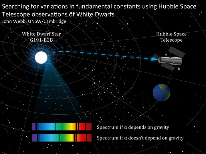
Searching for varia.ons in fundamental constants using Hubble Space Telescope observa.ons of White Dwarfs

John Webb, UNSW/Cambridge

• MaChew. Bainbridge (Leicester)

Mar.n Barstow (Leicester) Nicole Reindl (Leicester) John Barrow (Cambridge) John Webb (UNSW/Cambridge) Ji.ng Hu (UNSW) Simon Preval (Strathclyde) Jay Holberg (Arizona) Gillian Nave (NIST) Lydia Tchang-Brillet (Paris) Tom Ayres (Colorado)

Summary of this talk:

• Preliminary analysis described in Berengut et al 2013 (B13):
• New analyses of several WD spectra using FeV absorp.on
• FeV sample stringently filtered from max. of 750 transi.ons
• Each absorp.on profile Voigt profile fiCed
• Six tests made for poten.al systema.cs (including isotopic varia.ons, long-

range spectral distor.ons, Zeeman and Stark shi_s.

• None so far emulate the apparently non-zero result.

Results so far:

• 1. Eckberg 1975 wavelengths: Δα/α(G191-B2B) = 4.07 ± 0.47 x 10-5

Kramida 2014 wavelengths: Δα/α(G191-B2B) = 2.95 ± 0.53 x 10-5

• 2. Bd+28 gives similar results, consistent with the G191-B2B
• 3. Several other preliminary measurements also give non-zero
• 4. Systema.cs have not yet been fully quan.fied so treat the results with

skep.cism! Dominant error is lab wavelength uncertain.es (about 1 x 10-5).

Changing physics near massive bodies:

• Gravity is so important on large scales because it is addi.ve

(more par.cles = more gravity).

• Scalar fields couple to gravity.
• Therefore massive bodies should also impact on scalar fields.
• Varia.on in any standard model parameters are expressed in

terms of varia.ons in a scalar field (e.g. the dilaton, a hypothe.cal par.cle in the scalar field in string models and models with extra dimensions).

• Thus it would seem natural that fundamental constants vary

near massive bodies.

• 1. Damour & Polyakov, Nucl. Phys. B 423, 532 (1994) (arXiv:hep-th/9401069)
• 2. Flambaum & Shuryak, 2008, Nuclei and Mesoscopic Physic - WNMP 2007, 995, 1

(arXiv:physics/0701220v2)

• 3. Magueijo, Barrow, Sandvik, Physics LeCers B, Volume 549, Issue 3-4, p. 284-289

(arXiv:astro-ph/0202374)

Why white dwarfs?

• 1. GM/r at the photosphere is ~10,000 .mes greater than on

Earth

• 2. They are rela.vely bright objects so we can get high quality

spectra (although only in the UV and therefore from space)

• 3. There are many narrow spectral lines from species that are

sensi.ve to a change in the electromagne.c coupling constant

hCp://cronodon.com/

G191-B2B

HST STIS spectra of G191-B2B. Line widths ~4 km/s. Spectral resoluLon ~120,000

First WD varying constant measurement

• Phys. Rev. LeR. 111, 010801, 2013, arXiv:1305.1337

Limits on variaLons of the fine-structure constant with gravitaLonal potenLal from white-dwarf spectra

Berengut et al, arXiv:1305.1337

• White dwarf G191-B2B, ≈ 45 pc
• M = 0.51M⊙, R = 0.022R⊙
• ∆φ ~ 105 larger than terrestrial, “medium strength φ”
• HST/STIS spectra, R ≈ 144, 000
• Lab wavelength precision ~7mA (from residuals)
• Many FeV and NiV lines (~100) – helpful for some

systema.cs cf. quasar data

• Higher ioniza.on lines => sensi.vity coefficients higher

Parameterize sensi.vity of each transi.on frequency to a change: in α: Observed spectral lines are shi_ed due to

• 1. Doppler mo.on of star
• 2. Gravita.onal redshi_
• 3. Any possible dependence of α on Φ

where a small change in α is described by Rela.ng the laboratory wavelength to the observed wavelength in the WD photosphere: Where is the rela.ve sensi.vity of the transi.on frequency to a change in α

0.03 0.04 0.05 0.06 0.07 0.08 0.09 0.10 0.11 0.12 0.13 0.00007 0.00008 0.00009 0.00010

QΑ ΛΛ

FeV (blue circles) and NiV (red squares). Slopes of the lines give: ∆α/α = (4.2 ± 1.6) × 10−5 for FeV ; ∆α/α = (−6.1 ± 5.8) × 10−5 for Ni V The above plot does not make much sense!

Clearly there is something wrong in previous figure. The two sets of points should coincide. Yet ∆α/α = (4.2 ± 1.6) × 10−5 for FeV ; ∆α/α = (−6.1 ± 5.8) × 10−5 for Ni V Where’s the mistake?

• Laboratory wavelengths wrong?
• Maybe. But observed mean residuals are 0.03mA compared to

published wavelength errors of 0.04mA, sugges.ng not.

• Nonlinear wavelength distor.ons (i.e. incorrect calibra.on

between real and observed wavelength)?

• Maybe. To be determined.

1200 1300 1400 1500 1600 0.00007 0.00008 0.00009 0.00010

Λ0 ΛΛ

FeV (blue circles) and NiV (red squares). Note the different wavelength coverage for the 2 species. A “double”-linear wavelength distor.on, with a change in slope around 1350A could emulate varying alpha (but ruled out – later)

New analysis - Instead of using line centroids, model each individual absorpLon line with a Voigt profile Define chi-squared Taylor series expand it Therefore have to calculate derivaLves

But the first term averages to zero so we can ignore it and get a simple equa.on to solve! Which in prac.ce is modified slightly by introducing another free parameter p that enables more efficient minimisa.on

Second derivaLves

• f chi-squared

First derivaLves of chi-squared Discard first term Keep this one

Laboratory wavelength data: Eckberg 1975 and re-calibra.ons of Eckberg’s data by Kramida 2014 Nominally 4mÅ wavelength uncertain.es (although not a random error – see later slide) Plus new laboratory measurements (2 independent laboratories) Why FeV? There are lots of lines with a broad q-range Why not NiV or other species? Fewer NiV lines. Lab wavelength uncertain.es considerably worse Conserva.ve approach: Stringent absorp.on line sample selec.on:

• The Kentucky atomic database lists #12,364 electric dipole (E1) transi.ons (all

species) in the range 1160<λ<1680Å (range corresponding to HST STIS E140H)

• Of these 750 are FeV
• We minimise blends by selec.ng FeV lines without any other E1 transi.ons nearby

We therefore:

• 1. Detect all lines in the WD spectrum above 3σ limit
• 2. Iden.fy all electric dipole E1 transi.ons in the Kentucky atomic database sa.sfying
• 3. Accept line if there is only one iden.fica.on sa.sfying the condi.on above,
• therwise exclude (typical blend criterion is 3 km/s).

|λobs − λK| p σ(λobs)2 + σ(λK)2 ≤ 3

Astronomical and laboratory data used:

Test 1. The effect of random laboratory wavelength errors

• Simulate spectrum using {lab λs; the observed FeV line strengths; Δα/α = 4.1 × 10-5

(the observed value)}

• Add noise matching the real spectrum (and convolve to match STIS E140H)
• Add random uncertain.es to the lab λs (in atom.dat)
• Measure Δα/α in the simulated spectrum (VPFIT)
• Repeat 1000 .mes.

A B C D

TEST <Δα Δα/α> (x10-5) σ(< (<Δα Δα/α>) >) (x10-5) <χn

2>

σ(< (<χn

2>)

>) # of trials with χn

2<1.15

1.15 4mÅ (1000) 1.66 0.17 2mÅ (1000) 3.84 1.24 1.21 0.05 159 2mÅ (159) 3.78 1.27 1.13 0.02 159

Interpreta.on of 1.27 for 159 trials: distribu.on is comparable to the full 1000

• trials. This supports an error of about 2mÅ and shows the approach is plausible.

Conclusions are: (i) The data rule out random lab uncertain.es of 4mÅ (ii) The data marginally permit random lab uncertain.es of up to 2mÅ (iii) Assuming 2mÅ random uncertain.es, we could accommodate a systema.c uncertainty on Δα/α of about 1.3 × 10-5 (iv) This strongly moLvates improving the lab wavelengths.

Test 1. The effect of random laboratory wavelength errors

Test 2. Simple linear wavelength distorLon

Applying this distorLon makes α deviate further from terrestrial: Δα/α goes from 4.1 ± 0.47 × 10-5 (no distorLon correcLon), to Δα/α = 5.4 ± 0.46 × 10-5 (applying linear distorLon

• f 0.5 m/s/Å

Range of models tried

Best fit distor.on model, 0.5 m/s/Å Forcing α to the terrestrial value requires a massive distor.on, -14 m/s/Å, ruled out by the data itself

Test 3. Varying the Fe isotopic relaLve abundances

Simula.on parameters: 10-4 Å/pixel, b=2 km/s A B C D

Test 4. Randomly re-assign α-sensiLvity coefficients (q)

Randomise q’s over the whole sample 1000 trials Δα/α = -1.02 ± 11.87 × 10-6 Or, error on mean (rather than dispersion): -1.02e-6 ± 0.38 × 10-6 Global randomisa.on suggests things are working as expected

• 5

x10 2 0 4 0 6 0 8 0 100 120 140 160 180

• 4.0
• 3.5 -3.0
• 2.5 -2.0 -1.5
• 1.0 -0.5

0.0 0.5 1.0 1.5 2.0 2.5 3.0 3.5 delta_alpha Count randomlized q for all transition lines

A refinement of this: Perhaps more informa.vely: Randomise q’s within limited wavelength range about each line, i.e. allow for misiden.fica.ons (if present at all) to be local, rather than global). Not yet done.

Test 5. IteraLvely remove most discrepant FeV line

White: G191-B2B (36 lines) Red: Synthe.c (36 lines) Blue: G191-B2B (33 lines) Yellow: Synthe.c (33 lines) Why 36 33? 3 points appear to cause a sharp drop around f=0.6 and thus may be “spurious”

Test 6. IteraLvely remove least discrepant FeV line

White: G191-B2B (36 lines) Red: Synthe.c (36 lines)

Closing remarks:

We have apparent non-zero results from several white dwarf photospheres. Proper accoun.ng for systema.cs is incomplete, so non-zero results should be considered as upper limits at present. Laboratory wavelengths are par.cularly troublesome. But we now have 2 new independent experiments (NIST and Paris) AND in any case can look at changes in alpha from one WD to another Nevertheless we are closing in on a very good understanding of all systema.cs New Hubble Space Telescope STIS data is being collected this

• bserving cycle. 10-12 independent measurements on a .mescale
• f about a year