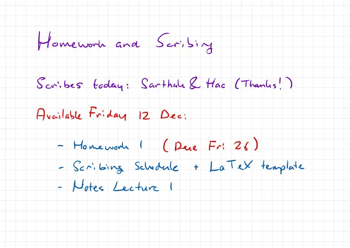
Scribing and ! ) & Scribes Sarthah Hao ( today Thanks ; - PowerPoint PPT Presentation

Homework Scribing and ! ) & Scribes Sarthah Hao ( today Thanks ; Friday Available Dec 12 ; ) ( Homework I Fri Due 26 - LATEX template Scribing Schedule + - Notes Lecture 1 -

Distribution Prior Posterior Recap ! and ,p# Density Biased ) Example Coin tl :p , : trim Prior Be } O ,,a( a y[ 's "m)=Beta( O ;o+a,p+b ) PLO Likelihood o , Binom ;a( ( a=§ ,yn ~ b=N a . , ( Sufficient Statistics ) Prior I Trial Trials to Trials loco -672 b=3Z8 , 'll ) Yi :( 0 0,1 ,o,l a y = , :b PLO )= ) ) Oiyiiiooo Oly , ) O p( p( ;y , :b p( = Betalo =Beta( 0,674,330 ) Betalo , 3 ) Betalb ; 6,4 ) ) ;2i2 ;2

distribution functions over Bayesian Regression / " ' i diggllloise dist ' f. fnpc f) fcxn ) - ,N En n=1 + En~ PIE yn = ... , ⇒ of Basis Function Linear • a fix f- ) ' • . • • x x I=×w = Iwaka D ×=tI÷El} := fCInl÷ f ( In ) Tvtocxn ) It In D= ' D t.ae#=t9tEIII1NX1NxDpxl - "

Polynomial Example Basis : Wttcfkn ) w°~p( I N ) En ) I t En~ PIE yn n= = ... , , 4 Reduces linear when ¢ to identity is reg . Polynomial Basis xD ¢d(×n ) = Prior in implies on f functions prior on

Over fitting Under fitting and - Under fitting Residuals strongly are correlated Over fitting Poor generalization

Ridge Regression ( Regularization ) LZ ia¥ TEI [ Objective : = IF cyn .it ' wto + wa . , I I=i I = o 10 =

¢( In Ridge Probabilistic Regression Interpretation : Normal ( Wd~ ~ s ) En It 1 En does + yn o not = , depend Normal ( uiiofkn ) ) Normal ( ) , 6) one 0,6 yn E. log plyntw ~ Maximum Posteriori a Est.mat@l5tkPH5lPl5largmwaxpcwl51-arggnaxpC5.w arynfax log piyii ) ) = " ( log is µ monotonic log + log pews pl 5,5 ) ) = logfntrs ignore = £ Normal ( x can ; M 6) - I ¥E , Phil log . ) 'M%2 ⇐ IK - ae = , = § , legato wtocxn - { )2 ( Yn . ) §e ) , log . ) pcynlw e-

= Itoki Ridge Probabilistic Regression Interpretation : Norm ,÷ [TEl=n§ if .cyn wto.si + . . Maximum Posteriori Estimation a Wd~ En~µorm( 0,6 ) ( o ) S ) En t yn , µ Depends log + log E. log plynliu pl 5,5 ) ) pw ) any an = and 6 s N tzsf D y . ztz § w¢( In ))2 woi ( yn t.co/nst = - - =L =L n Lridtelw 62 I piyii ) leg ) argngin arggmax = I =

Ridge Regression it Tcfkn ) s Norm Wd En~µorm( 0,6 ) ( ) En 0,5 t ~ yn = log piwly ) argugax 7=5--10 7=5--1 9=91--0 IEN I ( observations ) # [ woi ) 6 precise → o E [ En2]= 10 uninformative prior ) ( s → as

Posterior Predictive Distribution ( 3h55 Y } Yi yz ° Small o o 00 7=5 # y SZ ( 0 ° ooo # y ( o Large 0 000 A # y y* Posterior ( f f y* ) ) ) flx* pcy 1 1 Yi p previous ~ ~ :5 given observations

Posterior Predictive Distribution ,*y* hi µ f* € | . 5h55 l Y } y , yz , ° Small o o oo i 7=91 f " 0 l o o co 1 , # y * f , 0 1 Large 0 ooo 9 # y y* distribution ( kernel Lidge f*= 4*14 :µ ) E[ P(y*ly :X , ) ) pcytlfspcfly df = :n , , , Process ) regression ) ( full Gaussian :

Regression 515 Kennels Motivation with : N ? features What lots D Idea > > of if used we : 4*14=5 - ;) . 5 [%¥% TQ 5 E wtokn ) En + + yn = = µ " Rabab * * T 14=5 calculate Want to , = |dy*d5 > pcytlwlpiwl E[ 51 ) y* L to When Gaussian posterior |do ) pail : 4*16=0 F- [ 51 - = ] E[ d. |dI = angjnaxplw 15 ) wt¢(x* ) ) pc = WTI § ' ( take for ) =y ] , [ ) ¢k* # given as now =

Regression Kennels Motivation with : N ? features What lots D Idea > > of if used we : - . t.FI?. ) 5 TQ 5 E wtokn ) En + + yn = = * , an • nasa . f* E[ 4*14=5 ] 6*+46*1 o =z#tCy = = Solve tuwmf by )+7ws4→ 5,6 log I * ) derivative pc y = ungngnax I wrt 1 5- Easily iwtw - OI E) + = angmoax oIt5=#oI+i)w* d . Que 't

Regression Kennels Motivation with : N ? features What lots D Idea > > of if used we : - . 5 |%¥,¥,. ) TQ 5 E wtokn ) En + + yn = = pµ " pnxbab R DENY Dgt ' ya • d t.IT#ty )w' * # ( It ui* → = 01+5=0+01+71 Ridge regression : | Alternative matrix invert Dxb formal at '~ ' b×µ Dxt µ xD ) OIT (0101++91) 0(µ3 " II ) "0It ( OITOI + better = is O(p3 ) than Invert N×N matrix when N D > >

Kernel The Trick OIOIT CKIMQKI K I. stock ) ) ¢( = = | quit .io#i...ocxIiocxxi/ ... Idea kernel function use : 4655445 h( , Ej xi ;) ) := Expected value ( 1<+91515 f* # o*= ¢(I*stw* = ( 1<+9+-515 =(¢(E*st¢t ) Never need ( k+I±sInym } to computed In # hcE* = ,

kernel Ridge Regression 5=14 Yn ) * ' f li ' ' ' ' ( k ' , Its , g + = ( In ,Im be Knm ) = ten lr ( I* In ) = ,