Scheduling Algorithms of deciding which process in ready queue - - PDF document

2/15/2011 1

Gursharan Singh Tatla

professorgstatla@gmail.com

Scheduling Algorithms

15-Feb-2011 1 www.eazynotes.com

Scheduling Algorithms

 CPU Scheduling algorithms deal with the problem

• f deciding which process in ready queue should

be allocated to CPU.

 Following are the commonly used scheduling

algorithms:

15-Feb-2011 2 www.eazynotes.com

Scheduling Algorithms

15-Feb-2011 www.eazynotes.com 3

 First-Come-First-Served (FCFS)  Shortest Job First (SJF)  Priority Scheduling  Round-Robin Scheduling (RR)  Multi-Level Queue Scheduling (MLQ)  Multi-Level Feedback Queue Scheduling (MFQ)

First-Come-First-Served Scheduling (FCFS)

15-Feb-2011 www.eazynotes.com 4

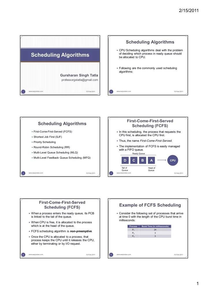
 In this scheduling, the process that requests the

CPU first, is allocated the CPU first.

 Thus, the name First-Come-First-Served.  The implementation of FCFS is easily managed

with a FIFO queue.

D C B A

CPU

T ail of Queue Head of Queue Ready Queue

15-Feb-2011 www.eazynotes.com 5

 When a process enters the ready queue, its PCB

is linked to the tail of the queue.

 When CPU is free, it is allocated to the process

which is at the head of the queue.

 FCFS scheduling algorithm is non-preemptive.  Once the CPU is allocated to a process, that

process keeps the CPU until it releases the CPU, either by terminating or by I/O request.

First-Come-First-Served Scheduling (FCFS)

Example of FCFS Scheduling

15-Feb-2011 www.eazynotes.com 6

 Consider the following set of processes that arrive

at time 0 with the length of the CPU burst time in milliseconds:

Process Burst Time (in milliseconds) P1 24 P2 3 P3 3

2/15/2011 2 Example of FCFS Scheduling

15-Feb-2011 www.eazynotes.com 7

 Suppose that the processes arrive in the order:

P1, P2, P3.

 The Gantt Chart for the schedule is:  Waiting Time for P1 = 0 milliseconds  Waiting Time for P2 = 24 milliseconds  Waiting Time for P3 = 27 milliseconds

P1 P2 P3 24 27 30 P1 24 P2 3 P3 3

Example of FCFS Scheduling

15-Feb-2011 www.eazynotes.com 8

 Average Waiting Time = (Total Waiting Time) /

• No. of Processes

= (0 + 24 + 27) / 3 = 51 / 3 = 17 milliseconds

Example of FCFS Scheduling

15-Feb-2011 www.eazynotes.com 9

 Suppose that the processes arrive in the order:

P2, P3, P1.

 The Gantt chart for the schedule is:  Waiting Time for P2 = 0 milliseconds  Waiting Time for P3 = 3 milliseconds  Waiting Time for P1 = 6 milliseconds

P1 P3 P2 6 3 30

Example of FCFS Scheduling

15-Feb-2011 www.eazynotes.com 10

 Average Waiting Time = (Total Waiting Time) /

• No. of Processes

= (0 + 3 + 6) / 3 = 9 / 3 = 3 milliseconds

 Thus, the average waiting time depends on the

• rder in which the processes arrive.

15-Feb-2011 www.eazynotes.com 11

 In SJF, the process with the least estimated execution

time is selected from the ready queue for execution.

 It associates with each process, the length of its next

CPU burst.

 When the CPU is available, it is assigned to the

process that has the smallest next CPU burst.

 If two processes have the same length of next CPU

burst, FCFS scheduling is used.

 SJF algorithm can be preemptive or non-preemptive.

Shortest Job First Scheduling (SJF)

Non-Preemptive SJF

15-Feb-2011 www.eazynotes.com 12

 In non-preemptive scheduling, CPU is assigned

to the process with least CPU burst time.

 The process keeps the CPU until it terminates.  Advantage:  It gives minimum average waiting time for a given

set of processes.

 Disadvantage:  It requires knowledge of how long a process will run

and this information is usually not available.

2/15/2011 3 Preemptive SJF

15-Feb-2011 www.eazynotes.com 13

 In preemptive SJF, the process with the smallest

estimated run-time is executed first.

 Any time a new process enters into ready queue,

the scheduler compares the expected run-time of this process with the currently running process.

 If the new process’s time is less, then the

currently running process is preempted and the CPU is allocated to the new process.

Example of Non-Preemptive SJF

15-Feb-2011 www.eazynotes.com 14

 Consider the following set of processes that arrive

at time 0 with the length of the CPU burst time in milliseconds:

Process Burst Time (in milliseconds) P1 6 P2 8 P3 7 P4 3

Example of Non-Preemptive SJF

15-Feb-2011 www.eazynotes.com 15

 The Gantt Chart for the schedule is:  Waiting Time for P4 = 0 milliseconds  Waiting Time for P1 = 3 milliseconds  Waiting Time for P3 = 9 milliseconds  Waiting Time for P2 = 16 milliseconds

P4 P3 P2 9 16 24 P1 3 P1 6 P2 8 P3 7 P4 3

Example of Non-Preemptive SJF

15-Feb-2011 www.eazynotes.com 16

 Average Waiting Time = (Total Waiting Time) /

• No. of Processes

= (0 + 3 + 9 + 16 ) / 4 = 28 / 4 = 7 milliseconds

Example of Preemptive SJF

15-Feb-2011 www.eazynotes.com 17

 Consider the following set of processes. These

processes arrived in the ready queue at the times given in the table:

Process Arrival Time Burst Time (in milliseconds) P1 8 P2 1 4 P3 2 9 P4 3 5

Example of Preemptive SJF

15-Feb-2011 www.eazynotes.com 18

 The Gantt Chart for the schedule is:  Waiting Time for P1 = 10 – 1 – 0 = 9  Waiting Time for P2 = 1 – 1 = 0  Waiting Time for P3 = 17 – 2 = 15  Waiting Time for P4 = 5 – 3 = 2

P1 P1 P4 1 17 10 P3 26 P2 5 P AT BT P1 8 P2 1 4 P3 2 9 P4 3 5

2/15/2011 4 Example of Preemptive SJF

15-Feb-2011 www.eazynotes.com 19

 Average Waiting Time = (Total Waiting Time) /

• No. of Processes

= (9 + 0 + 15 + 2) / 4 = 26 / 4 = 6.5 milliseconds

Explanation of the Example

15-Feb-2011 www.eazynotes.com 20

 Process P1 is started at time 0, as it is the only

process in the queue.

 Process P2 arrives at the time 1 and its burst time

is 4 milliseconds.

 This burst time is less than the remaining time of

process P1 (7 milliseconds).

 So, process P1 is preempted and P2 is scheduled.

Explanation of the Example

15-Feb-2011 www.eazynotes.com 21

 Process P3 arrives at time 2. Its burst time is 9

which is larger than remaining time of P2 (3 milliseconds).

 So, P2 is not preempted.  Process P4 arrives at time 3. Its burst time is 5.

Again it is larger than the remaining time of P2 (2 milliseconds).

 So, P2 is not preempted.

Explanation of the Example

15-Feb-2011 www.eazynotes.com 22

 After the termination of P2, the process with

shortest next CPU burst i.e. P4 is scheduled.

 After P4, processes P1 (7 milliseconds) and then

P3 (9 milliseconds) are scheduled.

Priority Scheduling

15-Feb-2011 www.eazynotes.com 23

 In priority scheduling, a priority is associated with

all processes.

 Processes are executed in sequence according

to their priority.

 CPU is allocated to the process with highest

priority.

 If priority of two or more processes are equal than

FCFS is used to break the tie.

Priority Scheduling

15-Feb-2011 www.eazynotes.com 24

 Priority scheduling can be preemptive or non-

preemptive.

 Preemptive Priority Scheduling:  In this, scheduler allocates the CPU to the new process if the priority of new process is higher tan the priority of the running process.  Non-Preemptive Priority Scheduling:  The running process is not interrupted even if the new process has a higher priority.  In this case, the new process will be placed at the head

• f the ready queue.

2/15/2011 5 Priority Scheduling

15-Feb-2011 www.eazynotes.com 25

 Problem:  In certain situations, a low priority process can be

blocked infinitely if high priority processes arrive in the ready queue frequently.

 This situation is known as Starvation.

Priority Scheduling

15-Feb-2011 www.eazynotes.com 26

 Solution:  Aging is a technique which gradually increases the

priority of processes that are victims of starvation.

 For e.g.: Priority of process X is 10.  There are several processes with higher priority in

the ready queue.

 Processes with higher priority are inserted into

ready queue frequently.

 In this situation, process X will face starvation.

Priority Scheduling

15-Feb-2011 www.eazynotes.com 27

(Cont.):

 The operating system increases priority of a

process by 1 in every 5 minutes.

 Thus, the process X becomes a high priority

process after some time.

 And it is selected for execution by the scheduler.

Example of Priority Scheduling

15-Feb-2011 www.eazynotes.com 28

 Consider the following set of processes that arrive

at time 0 with the length of the CPU burst time in

• milliseconds. The priority of these processes is

also given:

Process Burst Time Priority P1 10 3 P2 1 1 P3 2 4 P4 1 5 P5 5 2

Example of Priority Scheduling

15-Feb-2011 www.eazynotes.com 29

 The Gantt Chart for the schedule is:  Waiting Time for P2 = 0  Waiting Time for P5 = 1  Waiting Time for P1 = 6  Waiting Time for P3 = 16  Waiting Time for P4 = 18

P BT Pr P1 10 3 P2 1 1 P3 2 4 P4 1 5 P5 5 2 P2 P5 P1 P3 P4 1 6 16 18 19

Example of Priority Scheduling

15-Feb-2011 www.eazynotes.com 30

 Average Waiting Time = (Total Waiting Time) /

• No. of Processes

= (0 + 1 + 6 + 16 + 18) / 5 = 41 / 5 = 8.2 milliseconds

2/15/2011 6

Another Example of Priority Scheduling

15-Feb-2011 www.eazynotes.com 31

 Processes P1, P2, P3 are the processes with their

arrival time, burst time and priorities listed in table below:

Process Arrival Time Burst Time Priority P1 10 3 P2 1 5 2 P3 2 2 1

Another Example of Priority Scheduling

15-Feb-2011 www.eazynotes.com 32

 The Gantt Chart for the schedule is:  Waiting Time for P1 = 0 + (8 – 1) = 7  Waiting Time for P2 = 1 + (4 – 2) = 3  Waiting Time for P3 = 2

P AT BT Pr P1 10 3 P2 1 5 2 P3 2 2 1 P1 P2 P3 P2 P1 1 2 4 8 17

Another Example of Priority Scheduling

15-Feb-2011 www.eazynotes.com 33

 Average Waiting Time = (Total Waiting Time) /

• No. of Processes

= (7 + 3 + 2) / 3 = 12 / 3 = 4 milliseconds

Round Robin Scheduling (RR)

15-Feb-2011 www.eazynotes.com 34

 In Round Robin scheduling, processes are

dispatched in FIFO but are given a small amount

• f CPU time.

 This small amount of time is known as Time

Quantum or Time Slice.

 A time quantum is generally from 10 to 100

milliseconds.

Round Robin Scheduling (RR)

15-Feb-2011 www.eazynotes.com 35

 If a process does not complete before its time

slice expires, the CPU is preempted and is given to the next process in the ready queue.

 The preempted process is then placed at the tail

• f the ready queue.

 If a process is completed before its time slice

expires, the process itself releases the CPU.

 The scheduler then proceeds to the next process

in the ready queue.

Round Robin Scheduling (RR)

15-Feb-2011 www.eazynotes.com 36

 Round Robin scheduling is always preemptive as

no process is allocated the CPU for more than

• ne time quantum.

 If a process’s CPU burst time exceeds one time

quantum then that process is preempted and is put back at the tail of ready queue.

 The performance of Round Robin scheduling

depends on several factors:

 Size of Time Quantum  Context Switching Overhead

2/15/2011 7

Example of Round Robin Scheduling

15-Feb-2011 www.eazynotes.com 37

 Consider the following set of processes that arrive

at time 0 with the length of the CPU burst time in milliseconds:

 Time quantum is of 2 milliseconds.

Process Burst Time P1 10 P2 5 P3 2

Example of Round Robin Scheduling

15-Feb-2011 www.eazynotes.com 38

 The Gantt Chart for the schedule is:  Waiting Time for P1 = 0 + (6 – 2) + (10 – 8) + (13 – 12)

= 4 + 2 + 1 = 7

 Waiting Time for P2 = 2 + (8 – 4) + (12 – 10)

= 2 + 4 + 2 = 8

 Waiting Time for P3 = 4

P BT P1 10 P2 5 P3 2 P1 P2 P3 P1 P2 P1 P2 P1 P1 2 6 10 12 13 4 8 15 17

Example of Round Robin Scheduling

15-Feb-2011 www.eazynotes.com 39

 Average Waiting Time = (Total Waiting Time) /

• No. of Processes

= (7 + 8 + 4) / 3 = 19 / 3 = 6.33 milliseconds

Multi-Level Queue Scheduling (MLQ)

15-Feb-2011 www.eazynotes.com 40

 Multi-Level Queue scheduling classifies the

processes according to their types.

 For e.g.: a MLQ makes common division between

the interactive processes (foreground) and the batch processes (background).

 These two processes have different response

times, so they have different scheduling requirements.

 Also, interactive processes have higher priority

than the batch processes.

Multi-Level Queue Scheduling (MLQ)

15-Feb-2011 www.eazynotes.com 41

 In this scheduling, ready queue is divided into

various queues that are called subqueues.

 The processes are assigned to subqueues,

based on some properties like memory size, priority or process type.

 Each subqueue has its own scheduling algorithm.  For e.g.: interactive processes may use round

robin algorithm while batch processes may use FCFS.

Multi-Level Queue Scheduling (MLQ)

15-Feb-2011 www.eazynotes.com 42

2/15/2011 8

Multi-Level Feedback Queue Scheduling (MFQ)

15-Feb-2011 www.eazynotes.com 43

 Multi-Level Feedback Queue scheduling is an

enhancement of MLQ.

 In this scheme, processes can move between

different queues.

 The various processes are separated in different

queues on the basis of their CPU burst times.

 If a process consumes a lot of CPU time, it is placed

into a lower priority queue.

 If a process waits too long in a lower priority queue, it

is moved into higher priority queue.

 Such an aging prevents starvation.

Multi-Level Feedback Queue Scheduling (MFQ)

15-Feb-2011 www.eazynotes.com 44

Multi-Level Feedback Queue Scheduling (MFQ)

15-Feb-2011 www.eazynotes.com 45

 The top priority queue is given smallest CPU time

quantum.

 If the quantum expires before the process terminates,

it is then placed at the back of the next lower queue.

 Again, if it does not complete, it is put to the last

priority queue.

 The processes in this queue runs on FCFS

scheduling.

 If a process becomes a victim of starvation, it is

promoted to the next higher priority queue.

46 15-Feb-2011 www.eazynotes.com