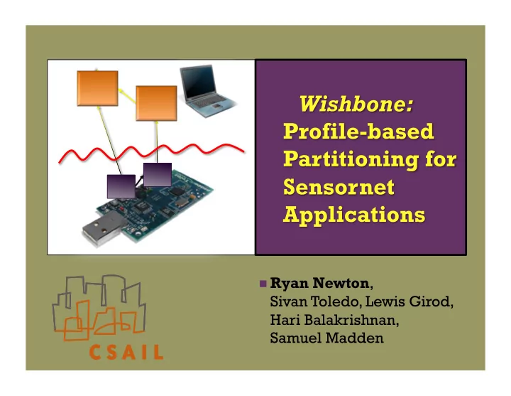
Ryan Newton , Sivan Toledo, Lewis Girod, Hari Balakrishnan, Samuel - PowerPoint PPT Presentation

 Ryan Newton , Sivan Toledo, Lewis Girod, Hari Balakrishnan, Samuel Madden

Example Application: Locating Marmots + 2 • Gothic, CO deployment August 2007 • Voxnet Platform • 2x PXA255, 64MB RAM, 8GB Flash, 802.11B, Mica2 supervisor, Li+ battery, Charge controller • Sensors: 4x48KHz audio, 3-axis accel, GPS, Internal temp with Lewis Girod & UCLA Blumstein Lab

+ We target sensing applications 3 Animal localization Pothole detection Computer Vision Pipeline leak detection Speaker identification EEG Seizure detection

+ Heterogeneous Platforms 4 Smartphones Low power sensors Router medium cpu, weak cpu/radio weak cpu, Contiki TinyOS strong radio strong radio JavaME Symbian Brew Android C++ Java Linux microserver Mix and Python Match! iPhone SDK

+ Contributions 5 Network Boundary Results Sensor source(s)

+ Contributions 6 Results Sensor source(s)

Contributions + Contributions 7 • First broadly portable sensenet programming • Partitioning algorithm • Optimize CPU/radio tradeoff even if Compile & Load app doesn’t “fit” Results Sensor source(s) Compile & Load

+ Architecture 8 Sample data (for profiling) Dataflow graph: operators containing code in portable Partitioner intermediate language Backend CodeGen Wishbone NesC/TinyOS JavaME ANSI C

+ Targeting TinyOS 9 • 16 bit microcontroller • 10K RAM • No mem. protection Task granularity, messaging model • No threads WaveScope : TinyOS : msg1 Execute! msg2 msg3 ( , ) f () f or () {…} g () Tasks t start t end time iterate x in S { f(); Profile-directed for(i=…) { Cooperative … Multitasking: } Same goal as g(); } Protothreads

+ Profiling Streams and Operators 10  Every sensor source is paired with sample data audioStream = 
 IFPROF(readFile(“foo8kHz”, 
 readSensor()))  Includes timing info  Measure rates, 20 Kbps 27 Kbps execution times 3 ms  Separately: profile network channel in deployment environment   per-node send rate

+ State, Replication, and Pinning 11 Pinning Constraints • All stateless ops: unpinned • Stateful replicated ops: unpinned • Stateful global ops: pinned to server – don’t distribute!

+ Problem Scenario 12 Embedded Node Server / Base Station 12 3 CPU: 19 7 11 Network: Problem Inputs 23 4 • profile data: net, cpu • network channel capacity NP-Hard Network Boundary

+ Partitioning Algorithm: 13 Integer linear program formulation f u � {0,1}  Introduce variables where 0=server, 1=sensor Tricky bit (see paper): 3 Parameters g uv � {0,1}  Introduce variables where 1 = cut edge Relating f and g while C, N, α staying linear  Enforce resource bounds cpu = f u ( compute u )  where cpu < C � u  where net < N net = g uv ( data uv ) � uv � Edges Proxy for  Minimize objective function Energy min( � ◊ cpu + net )

+ Evaluation: Two Applications 14 Human speech EEG-based seizure detection/identification onset detection source preemph hamming prefilt FFT filtbank logs cepstrals 1400 operators

+ Observation: 15 Relative cost varies by platform 1 Mote 0.9 N80 PC 0.8 Fraction of total CPU cost 0.7 0.6 Wishbone’s profiling visualizations 0.5 (via graphviz) for four platforms 0.4 0.3 0.2 0.1 0 source preemph hamming prefilt FFT filtBank logs cepstrals Operator

+ Visualizing Profile Data: 16 Bandwidth vs. Compute Execution time of operator (microseconds) Cumulative CPU Cost 50 Bandwidth (Right-hand scale) Bandwidth of cut (KBytes/Sec) Cumulative CPU cost (red) Processing reduces 1e+06 40 data quantity 100000 30 10000 1000 20 100 Reasonable 10 cutpoints 10 0 s p h p F f l c o i o l e r a r F t g e e u B p Operators: m T s e f r s a i c m l m t t n r e a i k p n l h s g

+ Optimal partitions across platforms 17 80 Number of operators in optimal node partition 70 60 50 40 30 20 10 TmoteSky/TinyOS NokiaN80/Java 0 0 2 4 6 8 10 12 14 16 18 20 Input data rate as a multiple of 8 kHz EEG Application (1 of 22 channels) Each line represents 2100 partioner-runs

+ Speaker Detection: CPU performance 18 across partitions/platforms 10000 TinyOS Handled input rate as multiple of 8 kHz Putting the pieces together: JavaME 1000 iPhone VoxNet • Cpu & net bounds  100 optimal partition (if exists) 10 • Partition  est. throughput 1 • Binary search over rates (aka cpu bounds)  0.1 max possible throughput 0.01 example: picks cutpoint after 0.001 filtBank for speaker detection source/1 filtbank/7 logs/8 cepstral/9 Cutpoint / number of operators in node partition Speaker Detection Application

+ Groundtruth: 19 Testbed deployment, 20 motes 5 1 TMote + Basestation 20 TMote Network How many detections can we actually get out of the network? 4 Detections per second 3 percent input events received percent network msgs successful goodput (product) 100 2 80 1 Percent 60 0 Best empirical source hamming FFT filtBank logs cepstral 40 Cutpoint cutpoint Compute/Bandwidth 20 Tension (1 mote + basestation) 0 source hamming FFT filtBank logs cepstral Cutpoint

+ Related Work 20  Graph partitioning for scientific codes  balanced, heuristic – e.g. Zoltan  Task scheduling, commonly list scheduling  Dynamic: Map-reduce, Condor, etc.  Sensor network context: Tenet and Vango  Linear pipeline of operators  Manual partition  Run TinyOS code on both server and sensor

+ 21 CONCLUSION

+ Partitioning: Algorithm Runtime 22 Time to discover optimal  Graph Preprocessing step Time to prove optimal  Merge vertices until all edge-weights are monotonically decreasing.  Eliminates the majority of edges  Even without preprocessing,  8000 runs, 0.1 1 10 100 1000 Seconds  partitioning the 1400-node EEG dataflow graph,  with different CPU budget,  took under 10 seconds 95% of the time.  But there is a long tail… luckily ILP solvers produce approximate solutions as well!

+ Motivating Example 23 budget = 2 budget = 3 budget = 4 5 5 5 5 5 5 1 1 1 1 1 1 4 4 4 4 4 4 2 2 2 2 2 2 1 1 1 1 1 1 bandwidth = 8 bandwidth = 6 bandwidth = 5 Unstable optimal partition. Flips between horizontal and vertical partition.