Routing Algorithms 14-740: Fundamentals of Computer Networks Bill - PowerPoint PPT Presentation
Routing Algorithms 14-740: Fundamentals of Computer Networks Bill Nace Material from Computer Networking: A Top Down Approach, J.F. Kurose and K.W. Ross Recall from Last Time Routing is the process of Routing creating and maintaining
Routing Algorithms 14-740: Fundamentals of Computer Networks Bill Nace Material from Computer Networking: A Top Down Approach, J.F. Kurose and K.W. Ross
Recall from Last Time • Routing is the process of Routing creating and maintaining Algorithm forwarding tables Forwarding Table Header Output value Link 0xx 3 100 1 101 2 11x 1 101 1 2 value in arriving 3 packet's header • Forwarding uses the table to determine the output link for each packet
traceroute • Routing Theory: Graphs and Overview • Link State Algorithms • Distance Vector Algorithms 3
Graph Abstraction • Internet is composed of routers/hosts connected with links • Can be modeled as a big graph • G = (N, E) • N = Set of routers • E = Set of links 4
Costs 5 v w 3 5 2 u z • c(N 1 ,N 2 ) = cost of the 2 3 1 1 2 link between N 1 ➙ N 2 x y 1 • ex: c(w, z) = 5, c(x,z) = ∞ • Cost could mean: 1 (hopcount), latency, congestion or inverse of bandwidth • Cost of path (N 1 , N 2 , .. N p ) = c(N 1 ,N 2 ) + c(N 2 , N 3 ) + .. + c(N p-1 ,N p ) 5
Routing 5 v w 3 5 2 u z • What is the least-cost 2 3 1 1 2 path between u and z? x y 1 • There are 17 di ff erent paths • Routing Algorithm: find the least-cost path between any pairs of nodes • When u forwards a packet bound for z : • Choose exit link with least-cost path 6
Algorithm Classifications • Global (“Link State” algorithms) • All routers have complete topology information and all link costs • Decentralized (“Distance Vector” algorithms) • Each router starts with just local knowledge • physically-connected neighbors • link costs to neighbors • Iterative process of computation, exchange of info with neighbors 7
traceroute • Routing Theory: Graphs and Overview • Link State Algorithms • Distance Vector Algorithms 8
Link State Algorithms • Use global knowledge: All routers know all • Connectivity, edge weights • How do all routers learn? Flooding • Each node sends its link-state information on all directly connected links • Each node relays such information on all of it’s links, etc 9
After the Flood • Each router calculates routes based on the link-state information • Deterministic algorithm, so each router comes up with same answer • Several algorithms exist: Dijkstra’s is most famous 10
Dijkstra’s Algorithm • Iterative algorithm • after k steps, know the least cost path to k closest locations • Notation • c(x,y): link cost from node x to y; ∞ if no direct link • D(v): current value of cost of path from source to node v • p(v): predecessor node along path from source to node v • N’: set of nodes whose least-cost path is known 11
Initialization: N' = {u} for all nodes v if v adjacent to u then D(v) = c(u,v) else D(v) = ∞ Loop until N' contains all nodes find w not in N' such that D(w) is a minimum add w to N' for all nodes v adjacent to w and ∉ N' D(v) = min( D(v), D(w) + c(w,v) ) /* new cost to v changes if path through w costs less */
5 v w Example 3 5 2 u z 2 3 1 1 2 x y 1 Step N’ D(v), p(v) D(w), p(w) D(x), p(x) D(y), p(y) D(z), p(z) 0 u 2, u 5, u 1, u ∞ ∞ 1 ux 2, u 4, x 2,x ∞ 2 uxy 2, u 3, y 4, y 3 uxyv 3, y 4, y 4 uxyvw 4, y 5 uxyvwz
Shortest Path Tree • For a graph G and a particular node r ... • ... the SPT( G , r ) is a tree... • ... with the shortest path from the root to any other node d in the graph A SPT for Europe (all roads lead to Rome)
Dijkstra’s Results • SPT ( G , u ) and a forwarding table for u destination link v w v v w x 2 u z 1 x x 1 2 x y y x 1 z x 15
Complexity • Algorithm complexity: n nodes xkcd.com/399 • each iteration: check all nodes not in N • first iteration, check n nodes • 2nd iteration, check n-1 nodes ... • Total is n(n+1)/2 comparisons ➙ O(n 2 ) • more e ffi cient implementations possible • Using a heap ➙ O(n log n) 16
traceroute • Routing Theory: Graphs and Overview • Link State Algorithms • Distance Vector Algorithms 17
Distance-Vector Algs • Still need to distribute local information • Message exchange rather than flooding • Each node exchanges distance vector with neighboring nodes • 1d map of nodes to distances 18
Routing Algorithm • Iterative: Each local iteration caused by .. • ... A change in local link cost • ... or DV update message from neighbor • Distributed • Each node autonomously computes based on local knowledge ... • ... which, after “enough” iterations is communicated to the world 19
Convergence • At each node: wait for change recompute estimates, based on change if DV to any destination has changed, notify neighbors • Convergence: process of getting consistent information to all nodes 20
Bellman-Ford Eqn • Define d x (y) as cost of the least-cost path from x to y • Bellman-Ford Equation says • d x (y) = min v {c(x,v) + d v (y)} • where min v means the min for all neighbors v of x xkcd.com/69 21
B-F Example 5 v w 3 5 2 u z • Neighbors of U: 2 3 1 • d v (z) = 5, d x (z) = 3, d w (z) = 3 1 2 x y 1 • d u (z) = min { c(u,v) + d v (z), c(u,x) + d x (z), c(u,w) + d w (z) } • d u (z) = min { 2 + 5, 1 + 3, 5 + 3 } = 4 • Node that achieves minimum is next hop in the shortest path • x goes in the forwarding table 22
Putting it all together • Each node periodically sends its own distance vector estimates to neighbors • When a node x receives a new DV estimate from a neighbor v , uses B-F • D x (y) ← min v {c(x,v)+D v (y)} for each y ∈ N • The estimate D x (y) converges to the actual d x (y) for minor, natural conditions 23
Example 5 v w 3 5 2 u z • At t=0 2 3 1 1 2 x y 1 Node U Node V Node W Node X Node Y Node Z ∞ ∞ u 0 u 2 u 5 u 1 u u v 2 v 0 v 3 v 2 v ∞ v ∞ w 5 w 3 w 0 w 3 w 1 w 5 ∞ x 1 x 2 x 3 x 0 x 1 x y ∞ y ∞ y 1 y 1 y 0 y 2 ∞ ∞ ∞ z z z 5 z z 2 z 0 24
Example 5 v w 3 5 2 u z • Node u receives DV 2 3 1 1 from w, v, x 2 x y 1 Node U Node V Node W Node X Node U(1) u 0 u 2 u 5 u 1 u 0 v 2 v 0 v 3 v 2 v 2 w 5 w 3 w 0 w 3 w 4 x 1 x 2 x 3 x 0 x 1 y ∞ y ∞ y 1 y 1 y 2 ∞ ∞ ∞ z z z 5 z z 10 d u (w) = min {c(u,u) + d u (w), c(u,v) + d v (w), c(u,w) + d w (w), c(u,x) + d x (w)} d u (w) = min {0 + 5, 2 + 3, 5 + 0, 1 + 3} d u (w) = 4 25
Example 5 v w 3 5 2 u z • After 1 exchange 2 3 1 1 2 x y 1 Node U Node V Node W Node X Node Y Node Z u 0 u 2 u 4 u 1 u 2 u 10 v 2 v 0 v v 2 v v 3 3 8 w 4 w 3 w 0 w 2 w 1 w 3 x 1 x 2 x 2 x 0 x 1 x 3 y y y y 1 y 0 y 2 3 1 2 z 10 z 8 z 3 z 3 z 2 z 0 26
Example 5 v w 3 5 2 u z • After 2 exchanges 2 3 1 1 2 x y 1 Node U Node V Node W Node X Node Y Node Z u 0 u 2 u 3 u 1 u 2 u 4 v 2 v 0 v v 2 v 3 v 3 5 w 3 w 3 w 0 w 2 w 1 w 3 x 1 x 2 x 2 x 0 x 1 x 3 y 2 y 3 y 1 y 1 y 0 y 2 z 4 z 5 z 3 z 3 z 2 z 0 27
Example 5 v w 3 5 2 u z • After 3 exchanges 2 3 1 1 2 x y 1 Node U Node V Node W Node X Node Y Node Z u 0 u 2 u 3 u 1 u 2 u 4 v 2 v 0 v 3 v 2 v 3 v 5 w 3 w 3 w 0 w 2 w 1 w 3 x 1 x 2 x 2 x 0 x 1 x 3 y 2 y 3 y 1 y 1 y 0 y 2 z 4 z 5 z 3 z 3 z 2 z 0 28
Dynamics • If a link cost changes • Node detects local link cost change, updates own forwarding table (recalculates DV) • If DV changes, will notify neighbors • “Good News travels fast” (one link-radius per exchange) 29
Dynamics (2) • But: Bad news travels slowly • If a link cost increases, can create a routing loop that slowly (and incorrectly) increases costs • “Count to Infinity” problem Y 60 • Ex: If link c(x,y) changes to 4 X 1 60, Z still thinks there is a 10 Z route to X of 5 30
In the Beginning Oh, no! A change occurs Result: X in 4 Result: X in 6 X in 4 Y Y Y 60 60 X in 4 X in 4 4 4 4 X X X 1 1 1 10 10 10 Z Z Z X in 10 X in 5 Result: X in 5 Result: X in 5 X in 5 Result: X in 6 Result: X in 8 Result: X in 8 Y Y Y 60 60 60 X in 6 X in 6 X in 8 4 4 4 X X X 1 1 1 10 10 10 Z Z Z X in 5 X in 7 X in 7 Result: X in 7 Result: X in 7 Result: X in 9 Finally, stability Result: X in 10 Result: X in 10 Result: X in 11 Y Y Y 60 60 60 X in 8 X in 10 X in 10 4 4 4 X X X 1 1 1 10 10 10 Z Z Z X in 9 X in 9 X in 10 Result: X in 9 Result: X in 10 Result: X in 10
Stabilization Techniques • Split horizon • When a node sends a routing update to its neighbor, does not send those routes it learned from each neighbor back to that neighbor • Split horizon with poisoned reverse • Nodes advertise a cost of ∞ for a destination to the neighbor it routes through to that destination 32
Example • Since Z routes through Y Y 60 to get to X, it tells Y that 4 X 1 D z (x) = ∞ 10 Z • D z (x) is actually 5 • Now, Y calculates D y (x) = min { 60, 1 + ∞ } • Y will tell Z that D y (x) = 60, so Z will calculate D z (x) = min {10, 1 + 60} 33
Recommend
More recommend
Explore More Topics
Stay informed with curated content and fresh updates.
