Review: probability Monty Hall, weighted dice Frequentist v. - PowerPoint PPT Presentation

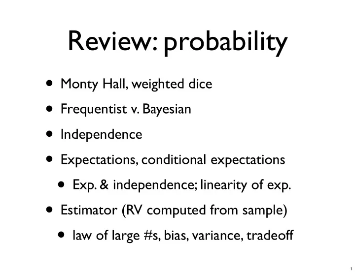
Review: probability • Monty Hall, weighted dice • Frequentist v. Bayesian • Independence • Expectations, conditional expectations • Exp. & independence; linearity of exp. • Estimator (RV computed from sample) • law of large #s, bias, variance, tradeoff 1

Covariance • Suppose we want an approximate numeric measure of (in)dependence • Let E(X) = E(Y) = 0 for simplicity • Consider the random variable XY • if X, Y are typically both +ve or both -ve • if X, Y are independent 2

Covariance • cov(X, Y) = • Is this a good measure of dependence? • Suppose we scale X by 10: 3

Correlation • Like covariance, but controls for variance of individual r.v.s • cor(X, Y) = • cor(10X, Y) = 4

Correlation & independence # • Equal probability ! on each point $ • Are X and Y Y " independent? ! $ • Are X and Y ! ! uncorrelated? ! # ! ! " ! X 5

Correlation & independence • Do you think that all independent pairs of RVs are uncorrelated? • Do you think that all uncorrelated pairs of RVs are independent? 6

Proofs and counterexamples ? • For a question A ⇒ B ? • e.g., X, Y uncorrelated ⇒ X, Y independent • if true, usually need to provide a proof • if false, usually only need to provide a counterexample 7

Counterexamples ? A ⇒ B ? X, Y uncorrelated ⇒ X, Y independent • Counterexample = example satisfying A but not B • E.g., RVs X and Y that are not independent, but are correlated 8

Correlation & independence # • Equal probability ! on each point $ • Are X and Y Y " independent? ! $ • Are X and Y ! ! uncorrelated? ! # ! ! " ! X 9

Rev. Thomas Bayes Bayes Rule 1702–1761 • For any X, Y, C • P(X | Y, C) P(Y | C) = P(Y | X, C) P(X | C) • Simple version (without context) • P(X | Y) P(Y) = P(Y | X) P(X) • Can be taken as definition of conditioning 10

Exercise • You are tested for a rare disease, emacsitis—prevalence 3 in 100,000 • Your receive a test that is 99% sensitive and 99% specific • sensitivity = P(yes | emacsitis) • specificity = P(no | ~emacsitis) • The test comes out positive • Do you have emacsitis? 11

Revisit: weighted dice • Fair dice: all 36 rolls equally likely • Weighted: rolls summing to 7 more likely • Data: 1-6 2-5 12

Learning from data • Given a model class • And some data, sampled from a model in this class • Decide which model best explains the sample 13

Bayesian model learning • P(model | data) = • Z = • So, for each model, compute: • Then: 14

Prior: uniform 0.25 0.2 0.15 0.1 0.05 0 0 0.2 0.4 0.6 0.8 1 all T all H 15

Posterior: after 5H, 8T 0.25 0.2 0.15 0.1 0.05 0 0 0.2 0.4 0.6 0.8 1 all T all H 16

Posterior:11H, 20T 0.25 0.2 0.15 0.1 0.05 0 0 0.2 0.4 0.6 0.8 1 all T all H 17

Graphical models 18

Why do we need graphical models? • So far, only way we’ve seen to write down a distribution is as a big table • Gets unwieldy fast! • E.g., 10 RVs, each w/ 10 settings • Table size = • Graphical model: way to write distribution compactly using diagrams & numbers 19

Example ML problem • US gov’t inspects food packing plants • 27 tests of contamination of surfaces • 12-point ISO 9000 compliance checklist • are there food-borne illness incidents in 30 days after inspection? (15 types) • Q: • A: 20

Big graphical models • Later in course, we’ll use graphical models to express various ML algorithms • e.g., the one from the last slide • These graphical models will be big! • Please bear with some smaller examples for now so we can fit them on the slides and do the math in our heads… 21

Bayes nets • Best-known type of graphical model • Two parts: DAG and CPTs 22

Rusty robot: the DAG 23

Rusty robot: the CPTs • For each RV (say X), there is one CPT specifying P(X | pa(X)) 24

Interpreting it 25

Benefits • 11 v. 31 numbers • Fewer parameters to learn • Efficient inference = computation of marginals, conditionals ⇒ posteriors 26

Inference example • P(M, Ra, O, W, Ru) = P(M) P(Ra) P(O) P(W|Ra,O) P(Ru|M,W) • Find marginal of M, O 27

Independence • Showed M ⊥ O • Any other independences? • Didn’t use • independences depend only on • May also be “accidental” independences 28

Conditional independence • How about O, Ru? O Ru • Suppose we know we’re not wet • P(M, Ra, O, W, Ru) = P(M) P(Ra) P(O) P(W|Ra,O) P(Ru|M,W) • Condition on W=F, find marginal of O, Ru 29

Conditional independence • This is generally true • conditioning on evidence can make or break independences • many (conditional) independences can be derived from graph structure alone • “accidental” ones are considered less interesting 30

Graphical tests for independence • We derived (conditional) independence by looking for factorizations • It turns out there is a purely graphical test • this was one of the key contributions of Bayes nets • Before we get there, a few more examples 31

Blocking • Shaded = observed (by convention) 32

Explaining away • Intuitively: 33

Son of explaining away 34

d-separation • General graphical test: “d-separation” • d = dependence • X ⊥ Y | Z when there are no active paths between X and Y • Active paths (W outside conditioning set): 35

Longer paths • Node is active if: and inactive o/w • Path is active if intermediate nodes are 36

Another example 37

Markov blanket • Markov blanket of C = minimal set of observations to render C independent of rest of graph 38

Learning Bayes nets P(M) = P(Ra) = P(O) = M Ra O W Ru P(W | Ra, O) = T F T T F T T T T T P(Ru | M, W) = F T T F F T F F F T F F T F T 39

Laplace smoothing P(M) = P(Ra) = P(O) = M Ra O W Ru P(W | Ra, O) = T F T T F T T T T T P(Ru | M, W) = F T T F F T F F F T F F T F T 40

Advantages of Laplace • No division by zero • No extreme probabilities • No near-extreme probabilities unless lots of evidence 41

Limitations of counting and Laplace smoothing • Work only when all variables are observed in all examples • If there are hidden or latent variables, more complicated algorithm—we’ll cover a related method later in course • or just use a toolbox! 42

Factor graphs • Another common type of graphical model • Uses undirected, bipartite graph instead of DAG 43

Rusty robot: factor graph P(M) P(Ra) P(O) P(W|Ra,O) P(Ru|M,W) 44

Convention • Don’t need to show unary factors • Why? They don’t affect algorithms below. 45

Non-CPT factors • Just saw: easy to convert Bayes net → factor graph • In general, factors need not be CPTs: any nonnegative #s allowed • In general, P(A, B, …) = • Z = 46

Ex: image segmentation 47

Factor graph → Bayes net • Possible, but more involved • Each representation can handle any distribution • Without adding nodes: • Adding nodes: 48

Independence • Just like Bayes nets, there are graphical tests for independence and conditional independence • Simpler, though: • Cover up all observed nodes • Look for a path 49

Independence example 50

Modeling independence • Take a Bayes net, list the (conditional) independences • Convert to a factor graph, list the (conditional) independences • Are they the same list? • What happened? 51