Reinforcement Learning Quentin Huys Division of Psychiatry and Max - - PowerPoint PPT Presentation

reinforcement learning
SMART_READER_LITE
LIVE PREVIEW

Reinforcement Learning Quentin Huys Division of Psychiatry and Max - - PowerPoint PPT Presentation

Reinforcement Learning Quentin Huys Division of Psychiatry and Max Planck UCL Centre for Computational Psychiatry and Ageing Research, UCL Complex Depression, Anxiety and Trauma Service, Camden and Islington NHS Foundation Trust Systems and


slide-1
SLIDE 1

Reinforcement Learning

Quentin Huys

Division of Psychiatry and Max Planck UCL Centre for Computational Psychiatry and Ageing Research, UCL Complex Depression, Anxiety and Trauma Service, Camden and Islington NHS Foundation Trust

Systems and Theoretical Neuroscience Course, 4/12/18

slide-2
SLIDE 2

Quentin Huys RL SWC

Setup

Sutton and Barto 2017

Environment Agent

at rt st

slide-3
SLIDE 3

Quentin Huys RL SWC

Setup

Sutton and Barto 2017

Environment Agent

at rt st

{at} ← argmax

{at} ∞

  • t=1

rt

slide-4
SLIDE 4

Quentin Huys RL SWC

Setup

Sutton and Barto 2017

Environment Agent

at rt st

{at} ← argmax

{at} ∞

  • t=1

rt

Minimizing Loss = Maximizing Reward

slide-5
SLIDE 5

Quentin Huys RL SWC

State space

Gold +1 Electric shocks

  • 1
slide-6
SLIDE 6

Quentin Huys RL SWC

A Markov Decision Problem

st ∈ S at ∈ A T a

ss

= p(st+1|st, at) rt ∼ R(st+1, at, st) π(a|s) = p(a|s)

slide-7
SLIDE 7

Quentin Huys RL SWC

A Markov Decision Problem

st ∈ S at ∈ A T a

ss

= p(st+1|st, at) rt ∼ R(st+1, at, st) π(a|s) = p(a|s)

slide-8
SLIDE 8

Quentin Huys RL SWC

A Markov Decision Problem

st ∈ S at ∈ A T a

ss

= p(st+1|st, at) rt ∼ R(st+1, at, st) π(a|s) = p(a|s)

slide-9
SLIDE 9

Quentin Huys RL SWC

Actions

1 2 3 4 5 6 7

Action left Action right

T right =           1 1 1 1 1 1 1           T left =           1 1 1 1 1 1 1          

slide-10
SLIDE 10

Quentin Huys RL SWC

Actions

1 2 3 4 5 6 7

Action left Action right

T right =           1 1 1 1 1 1 1           T left =           .8 .8 .2 .2 .8 .2 .8 .2 .8 .2 .8 .2 .8          

Noisy: plants, environments, agent

slide-11
SLIDE 11

Quentin Huys RL SWC

Actions

1 2 3 4 5 6 7

Action left Action right

T right =           1 1 1 1 1 1 1           T left =           .8 .8 .2 .2 .8 .2 .8 .2 .8 .2 .8 .2 .8          

Absorbing state -> max eigenvalue < 1

abs

Noisy: plants, environments, agent

slide-12
SLIDE 12

Quentin Huys RL SWC

Markovian dynamics

p(st+1|at, st, at−1, st−1, at−2, st−2, · · · ) = p(st+1|at, st)

Velocity

at−2, st−2 → at−1, st−1 → at, st

slide-13
SLIDE 13

Quentin Huys RL SWC

Markovian dynamics

p(st+1|at, st, at−1, st−1, at−2, st−2, · · · ) = p(st+1|at, st)

Velocity

at−2, st−2 → at−1, st−1 → at, st

slide-14
SLIDE 14

Quentin Huys RL SWC

Markovian dynamics

p(st+1|at, st, at−1, st−1, at−2, st−2, · · · ) = p(st+1|at, st)

Velocity

s = [position] → s = position velocity ⇥

at−2, st−2 → at−1, st−1 → at, st

slide-15
SLIDE 15

Quentin Huys RL SWC

A Markov Decision Problem

st ∈ S at ∈ A T a

ss

= p(st+1|st, at) rt ∼ R(st+1, at, st) π(a|s) = p(a|s)

slide-16
SLIDE 16

Quentin Huys RL SWC

A Markov Decision Problem

st ∈ S at ∈ A T a

ss

= p(st+1|st, at) rt ∼ R(st+1, at, st) π(a|s) = p(a|s)

slide-17
SLIDE 17

Quentin Huys RL SWC

A Markov Decision Problem

st ∈ S at ∈ A T a

ss

= p(st+1|st, at) rt ∼ R(st+1, at, st) π(a|s) = p(a|s)

  • 1

+1

slide-18
SLIDE 18

Quentin Huys RL SWC

Tall orders

  • Aim: maximise total future reward
  • i.e. we have to sum over paths through the

future and weigh each by its probability

  • Best policy achieves best long-term reward

X

t=1

rt

slide-19
SLIDE 19

Quentin Huys RL SWC

Exhaustive tree search

slide-20
SLIDE 20

Quentin Huys RL SWC

Exhaustive tree search

wd

slide-21
SLIDE 21

Quentin Huys RL SWC

Decision tree

X

t=1

rt

slide-22
SLIDE 22

Quentin Huys RL SWC

Decision tree

X

t=1

rt

8

slide-23
SLIDE 23

Quentin Huys RL SWC

Decision tree

X

t=1

rt

8 64

slide-24
SLIDE 24

Quentin Huys RL SWC

Decision tree

X

t=1

rt

8 64 512 ...

slide-25
SLIDE 25

Quentin Huys RL SWC

Policy for this talk

  • Pose the problem mathematically
  • Policy evaluation
  • Policy iteration
  • Monte Carlo techniques: experience samples
  • TD learning

Policy Update Evaluate

slide-26
SLIDE 26

Quentin Huys RL SWC

Evaluating a policy

  • Aim: maximise total future reward
  • To know which is best, evaluate it first
  • The policy determines the expected reward

from each state

Vπ(s1) = E " ∞ X

t=1

rt|s1 = 1, at ∼ π #

X

t=1

rt

slide-27
SLIDE 27

Quentin Huys RL SWC

Discounting

  • Given a policy, each state has an expected

value

  • But:
  • Episodic
  • Discounted
  • infinite horizons
  • finite, exponentially distributed horizons

  • t=0

γtrt < ∞

  • t=0

rt = ∞

T ∼ 1 τ et/τ

T

  • t=0

γtrt

Vπ(s1) = E " ∞ X

t=1

rt|s1 = 1, at ∼ π #

T

X

t=0

rt < ∞

slide-28
SLIDE 28

Quentin Huys RL SWC

Discounting

  • Given a policy, each state has an expected

value

  • But:
  • Episodic
  • Discounted
  • infinite horizons
  • finite, exponentially distributed horizons

  • t=0

γtrt < ∞

  • t=0

rt = ∞

T ∼ 1 τ et/τ

T

  • t=0

γtrt

Vπ(s1) = E " ∞ X

t=1

rt|s1 = 1, at ∼ π #

T

X

t=0

rt < ∞

slide-29
SLIDE 29

Quentin Huys RL SWC

Discounting

  • Given a policy, each state has an expected

value

  • But:
  • Episodic
  • Discounted
  • infinite horizons
  • finite, exponentially distributed horizons

  • t=0

γtrt < ∞

  • t=0

rt = ∞

T ∼ 1 τ et/τ

T

  • t=0

γtrt

Vπ(s1) = E " ∞ X

t=1

rt|s1 = 1, at ∼ π #

T

X

t=0

rt < ∞

slide-30
SLIDE 30

Quentin Huys RL SWC

Markov Decision Problems

This dynamic consistency is key to many solution approaches. It states that the value of a state s is related to the values of its successor states s’.

V π(st) = E " ∞ X

t0=1

rt0|st = s, π # = E [r1| st = s, π] + E " ∞ X

t=2

rt|st = s, π # = E [r1| st = s, π] + E [V π(st+1)|st = s, π]

slide-31
SLIDE 31

Quentin Huys RL SWC

Markov Decision Problems

V π(st) = E [r1| st = s, π] + E [V (st+1), π] r1 ∼ R(s2, a1, s1) E [r1|st = s, π] = E 2 4X

st+1

p(st+1|st, at)R(st+1, at, st) 3 5 = X

at

p(at|st) 2 4X

st+1

p(st+1|st, at)R(st+1, at, st) 3 5 = X

at

π(at, st) 2 4X

st+1

T at

stst+1R(st+1, at, st)

3 5

slide-32
SLIDE 32

Quentin Huys RL SWC

Bellman equation

V π(st) = E [r1| st = s, π] + E [V (st+1), π] E [r1|st, π] = X

a

π(a, st) 2 4X

st+1

T a

stst+1R(st+1, a, st)

3 5 E [V π(st+1), π, st] = X

a

π(a, st) 2 4X

st+1

T a

stst+1V π(st+1)

3 5

V π(s) = X

a

π(a|s) "X

s0

T a

ss0 [R(s0, a, s) + V π(s0)]

#

slide-33
SLIDE 33

Quentin Huys RL SWC

Bellman Equation

V π(s) = X

a

π(a|s) "X

s0

T a

ss0 [R(s0, a, s) + V π(s0)]

#

slide-34
SLIDE 34

Quentin Huys RL SWC

Bellman Equation

All future reward from state s Immediate reward = E All future reward from next state s’ +

V π(s) = X

a

π(a|s) "X

s0

T a

ss0 [R(s0, a, s) + V π(s0)]

#

slide-35
SLIDE 35

Quentin Huys RL SWC

Bellman Equation

All future reward from state s Immediate reward = E All future reward from next state s’ +

V π(s) = X

a

π(a|s) "X

s0

T a

ss0 [R(s0, a, s) + V π(s0)]

#

slide-36
SLIDE 36

Quentin Huys RL SWC

Q values = state-action values

  • so we can define state-action values as:
  • and state values are average state-action

values:

Q(s, a) = ⇤

s

T a

ss [R(s, a, s) + V (s)]

= E ⇥ ⇤

t=1

rt|s, a ⇥

V (s) =

  • a

π(a|s)Q(s, a)

V π(s) = X

a

π(a|s) "X

s0

T a

ss0 [R(s0, a, s) + V π(s0)]

# | {z }

Qπ(s,a)

slide-37
SLIDE 37

Quentin Huys RL SWC

Bellman Equation

  • to evaluate a policy, we need to solve the above

equation, i.e. find the self-consistent state values

  • options for policy evaluation
  • exhaustive tree search - outwards, inwards, depth-first
  • value iteration: iterative updates
  • linear solution in 1 step
  • sampling

V π(s) = X

a

π(a|s) "X

s0

T a

ss0 [R(s0, a, s) + V π(s0)]

#

slide-38
SLIDE 38

Quentin Huys RL SWC

Solving the Bellman Equation

Option 1: turn it into update equation Option 2: linear solution

V (s) = ⇤

a

π(a, st) ⇤

s

T a

ss [R(s⇥, a, s) + V (s⇥)]

⇥ ⇒ v = Rπ + Tπv ⇒ vπ = (I − Tπ)1Rπ

(w/ absorbing states)

O(|S|3)

slide-39
SLIDE 39

Quentin Huys RL SWC

Solving the Bellman Equation

V k+1(s) = ⇧

a

π(a, st) ⇤⇧

s

T a

ss

  • R(s, a, s) + V k(s)

⇥ ⌅

Option 1: turn it into update equation Option 2: linear solution

V (s) = ⇤

a

π(a, st) ⇤

s

T a

ss [R(s⇥, a, s) + V (s⇥)]

⇥ ⇒ v = Rπ + Tπv ⇒ vπ = (I − Tπ)1Rπ

(w/ absorbing states)

O(|S|3)

slide-40
SLIDE 40

Quentin Huys RL SWC

Policy update

Given the value function for a policy, say via linear solution Given the values V for the policy, we can improve the policy by always choosing the best action:

V π(s) = X

a

π(a|s) "X

s0

T a

ss0 [R(s0, a, s) + V π(s0)]

# | {z }

Qπ(s,a)

It is guaranteed to improve: Qπ(s, π0(s)) = max

a

Qπ(s, a) ≥ Qπ(s, π(s)) = Vπ(s)

for deterministic policy

π0(a|s) = ⇢ 1 if a = argmaxa Qπ(s, a) 0 else

slide-41
SLIDE 41

Quentin Huys RL SWC

Policy iteration

vπ = (I − Tπ)−1Rπ

Policy evaluation

π(a|s) = ⇤ 1 if a = argmaxa ⌅

s T a ss

  • Ra

ss + V pi(s)

⇥ 0 else

slide-42
SLIDE 42

Quentin Huys RL SWC

Policy iteration

vπ = (I − Tπ)−1Rπ

Policy evaluation greedy policy improvement

π(a|s) = ⇤ 1 if a = argmaxa ⌅

s T a ss

  • Ra

ss + V pi(s)

⇥ 0 else

slide-43
SLIDE 43

Quentin Huys RL SWC

Policy iteration

vπ = (I − Tπ)−1Rπ V (s) = max

a

  • s

T a

ss [Ra ss + V (s⇥)]

Policy evaluation greedy policy improvement Value iteration

π(a|s) = ⇤ 1 if a = argmaxa ⌅

s T a ss

  • Ra

ss + V pi(s)

⇥ 0 else

slide-44
SLIDE 44

Quentin Huys RL SWC

Model-free solutions

  • So far we have assumed knowledge of R and T
  • R and T are the ‘model’ of the world, so we assume full

knowledge of the dynamics and rewards in the environment

  • What if we don’t know them?
  • We can still learn from state-action-reward

samples

  • we can learn R and T from them, and use our

estimates to solve as above

  • alternatively, we can directly estimate V or Q
slide-45
SLIDE 45

Quentin Huys RL SWC

Solving the Bellman Equation

V (s) = ⇤

a

π(a, st) ⇤

s

T a

ss [R(s, a, s) + V (s)]

Option 3: sampling

a = X

k

f(xk)p(xk) x(i) ∼ p(x) → ˆ a = 1 N X

i

f(x(i))

So we can just draw some samples from the policy and the transitions and average over them:

slide-46
SLIDE 46

Quentin Huys RL SWC

Solving the Bellman Equation

Option 3: sampling

a = X

k

f(xk)p(xk) x(i) ∼ p(x) → ˆ a = 1 N X

i

f(x(i))

So we can just draw some samples from the policy and the transitions and average over them:

slide-47
SLIDE 47

Quentin Huys RL SWC

Solving the Bellman Equation

Option 3: sampling this is an expectation over policy and transition samples.

a = X

k

f(xk)p(xk) x(i) ∼ p(x) → ˆ a = 1 N X

i

f(x(i))

So we can just draw some samples from the policy and the transitions and average over them:

slide-48
SLIDE 48

Quentin Huys RL SWC

Solving the Bellman Equation

Option 3: sampling this is an expectation over policy and transition samples.

a = X

k

f(xk)p(xk) x(i) ∼ p(x) → ˆ a = 1 N X

i

f(x(i))

So we can just draw some samples from the policy and the transitions and average over them: more about this later...

slide-49
SLIDE 49

Quentin Huys RL SWC

Learning from samples

1 2 3 4 5 6 7 8 9 10 1 2 3 4 5 6 7 8 9 10

A new problem: exploration versus exploitation

slide-50
SLIDE 50

Quentin Huys RL SWC

The effect of bootstrapping

B1 B1 B1 B1 B1 B1 B0 A0 B0 Markov (every visit) V(B)=3/4 V(A)=0 TD V(B)=3/4 V(A)=~3/4

after Sutton and Barto 1998

  • Average over various bootstrappings: TD( )

λ

slide-51
SLIDE 51

Quentin Huys RL SWC

Monte Carlo

  • First visit MC
  • randomly start in all states, generate paths, average

for starting state only

  • More efficient use of samples
  • Every visit MC
  • Bootstrap: TD
  • Dyna
  • Better samples
  • on policy versus off policy
  • Stochastic search, UCT...

V(s) = 1 N X

i

( T X

t0=1

ri

t0|s0 = s

)

1 2 3 4 5 6 7 8 9 10 1 2 3 4 5 6 7 8 9 10

slide-52
SLIDE 52

Quentin Huys RL SWC

Update equation: towards TD

Bellman equation

V (s) = ⇤

a

π(a, s) ⇤

s

T a

ss [R(s, a, s) + V (s)]

Not yet converged, so it doesn’t hold: And then use this to update

V i+1(s) = V i(s) + dV (s) dV (s) = −V (s) + ⇤

a

π(a, s) ⇤

s

T a

ss [R(s, a, s) + V (s)]

slide-53
SLIDE 53

Quentin Huys RL SWC

TD learning

dV (s) = −V (s) + ⇤

a

π(a, s) ⇤

s

T a

ss [R(s, a, s) + V (s)]

slide-54
SLIDE 54

Quentin Huys RL SWC

TD learning

Sample

at ∼ π(a|st) st+1 ∼ T at

st,st+1

rt = R(st+1, at, st) dV (s) = −V (s) + ⇤

a

π(a, s) ⇤

s

T a

ss [R(s, a, s) + V (s)]

slide-55
SLIDE 55

Quentin Huys RL SWC

TD learning

Sample

at ∼ π(a|st) st+1 ∼ T at

st,st+1

rt = R(st+1, at, st) dV (s) = −V (s) + ⇤

a

π(a, s) ⇤

s

T a

ss [R(s, a, s) + V (s)]

⇥ δt = −Vt−1(st) + rt + Vt−1(st+1)

slide-56
SLIDE 56

Quentin Huys RL SWC

TD learning

V i+1(s) = V i(s) + dV (s)

Sample

at ∼ π(a|st) st+1 ∼ T at

st,st+1

rt = R(st+1, at, st) dV (s) = −V (s) + ⇤

a

π(a, s) ⇤

s

T a

ss [R(s, a, s) + V (s)]

⇥ Vt(st) = Vt−1(st) + αδt δt = −Vt−1(st) + rt + Vt−1(st+1)

slide-57
SLIDE 57

Quentin Huys RL SWC

TD learning

at ∼ π(a|st) st+1 ∼ T at

st,st+1

rt = R(st+1, at, st) δt = −Vt(st) + rt + Vt(st+1) Vt+1(st) = Vt(st) + αδt

slide-58
SLIDE 58

Quentin Huys RL SWC

Phasic dopamine neurone firing in

Montague et al., 1996, Schultz et al., 1997

  • Pavlovian conditioning
slide-59
SLIDE 59

Quentin Huys RL SWC

Phasic dopamine neurone firing in

Montague et al., 1996, Schultz et al., 1997

  • Pavlovian conditioning

Reward Reward Loss Reward

slide-60
SLIDE 60

Quentin Huys RL SWC

Phasic dopamine neurone firing in

Montague et al., 1996, Schultz et al., 1997

  • Pavlovian conditioning

Reward Reward Loss Reward

Vt+1(s) = Vt(s) + ✏ (Rt − Vt(s)) | {z }

= Prediction error

slide-61
SLIDE 61

Quentin Huys RL SWC

Phasic dopamine neurone firing in

Montague et al., 1996, Schultz et al., 1997

  • Pavlovian conditioning

Reward Reward Loss Reward

Vt+1(s) = Vt(s) + ✏ (Rt − Vt(s)) | {z }

= Prediction error

slide-62
SLIDE 62

Quentin Huys RL SWC

Phasic signals in humans

D’Ardenne et al., 2008 Science; Zaghloul et al., 2009 Science

* *

unexpected reward expected reward reward expected, not received

0.008 0.004

  • 0.004

Effect Size

B

NS

re- d

  • luster
slide-63
SLIDE 63

Quentin Huys RL SWC

Blocking

Kamin 1968

  • Are predictions and prediction errors really

causally important in learning?

  • 1: A -> Reward
  • 2: A+B -> Reward
  • 3: A -> ? approach
  • B -> ? approach

A B

Response

C

slide-64
SLIDE 64

Quentin Huys RL SWC

Causal role of phasic DA in learning

Steinberg et al., 2013 Nat. Neurosci.

b

Single Test cue A US AX US X? With paired or unpaired

  • ptical stimulation

Compound cue 14–15 d 4 d 1 d

c

Paired stimulation Unpaired stimulation Cue AX Time in port US (sucrose) +Stim Cue AX Time in port US (sucrose) Stim

**

P = 0.095 5 10 15 20 25 1 trial 3 trials Blocking (n = 12) Control (n = 11)

e

1 2 3

f

5 10 15

** *

PairedCre+ (n = 9) UnpairedCre+ (n = 9) P = 0.055 1 trial PairedCre− (n = 10) 3 trials

slide-65
SLIDE 65

Quentin Huys RL SWC

Markov Decision Problems

V (st) = E[rt + rt+1 + rt+2 + . . .] = E[rt] + E[rt+1 + rt+2 + rt+3 . . .] ⇒ V (st) = E[rt] + V (st+1)

slide-66
SLIDE 66

Quentin Huys RL SWC

“Cached” solutions to MDPs

slide-67
SLIDE 67

Quentin Huys RL SWC

“Cached” solutions to MDPs

  • Learn from experience
  • If we have true values V, then this is true every

trial:

  • If it is not true (we don’t know true V), then we

get an error:

  • So now we can update with our experience
  • This is an average over past experience

V (st) = E[rt] + V (st+1) V (st) ← V (st) + ✏ δ = (E[rt] + V (st+1)) V (st) 6= 0

slide-68
SLIDE 68

Quentin Huys RL SWC

SARSA

  • Do TD for state-action values instead:
  • convergence guarantees - will estimate

Q(st, at) ← Q(st, at) + α[rt + γQ(st+1, at+1) − Q(st, at)]

st, at, rt, st+1, at+1 Qπ(s, a)

slide-69
SLIDE 69

Quentin Huys RL SWC

Q learning: off-policy

  • Learn off-policy
  • draw from some policy
  • “only” require extensive sampling
  • will estimate

Q(st, at) ← Q(st, at) + α

  • ⇤rt + γ max

a

Q(st+1, a) ⌥ ⌃⇧

  • −Q(st, at)

⇥ ⌅

update towards

  • ptimum

Q∗(s, a)

slide-70
SLIDE 70

Quentin Huys RL SWC

MF and MB learning of V and Q values

Model-free Model-based Pavlovian (state) values VMF s ð Þ VMB s ð Þ Instrumental (state-action) values QMF s, a ð Þ QMB s, a ð Þ

There are both Pavlovian state and instrumental state-action values, and both of these can be either model-free (cached) or model-based.

slide-71
SLIDE 71

Quentin Huys RL SWC

Solutions

  • “Cached” learning
  • average experience
  • do again what worked in the past
  • averages are cheap to compute - no computational

curse

  • averages move slowly
  • “Goal-directed” or “Model-based” decisions
  • Think through possible options and choose the best
  • Requires detailed model of the world
  • Requires huge computational resources
  • Learning = building the model, extracting structure

If you have an average over large number of subjects, it won’t move much if you add one more.

slide-72
SLIDE 72

Quentin Huys RL SWC

Solutions

  • “Cached” learning
  • average experience
  • do again what worked in the past
  • averages are cheap to compute - no computational

curse

  • averages move slowly
  • “Goal-directed” or “Model-based” decisions
  • Think through possible options and choose the best
  • Requires detailed model of the world
  • Requires huge computational resources
  • Learning = building the model, extracting structure

If you have an average over large number of subjects, it won’t move much if you add one more.

slide-73
SLIDE 73

Quentin Huys RL SWC

MF and MB learning of V and Q values

Model-free Model-based Pavlovian (state) values VMF s ð Þ VMB s ð Þ Instrumental (state-action) values QMF s, a ð Þ QMB s, a ð Þ

There are both Pavlovian state and instrumental state-action values, and both of these can be either model-free (cached) or model-based.

slide-74
SLIDE 74

Quentin Huys RL SWC

Pavlovian and instrumental

  • Pavlovian model-free learning:
  • Instrumental model-free learning:

Vt(s) = Vt−1(s) + ✏(rt − Vt−1(s)) Qt(a, s) = Qt−1(a, s) + ✏(rt − Qt−1(a, s)) p(a|s, V) ∝ f(a, V(s)) p(a|s)

slide-75
SLIDE 75

Quentin Huys RL SWC

Innate evolutionary strategies

Hirsch and Bolles 1980

slide-76
SLIDE 76

Quentin Huys RL SWC

Innate evolutionary strategies

Hirsch and Bolles 1980

more survive more survive fewer survive

slide-77
SLIDE 77

Quentin Huys RL SWC

Innate evolutionary strategies

Hirsch and Bolles 1980

more survive more survive fewer survive

are quite sophisticated...

slide-78
SLIDE 78

Quentin Huys RL SWC

Unconditioned responses

Hershberger 1986

  • powerful
  • inflexible over short timescale
  • adaptive on evolutionary scale
slide-79
SLIDE 79

Quentin Huys RL SWC

Unconditioned responses

Hershberger 1986

  • powerful
  • inflexible over short timescale
  • adaptive on evolutionary scale
slide-80
SLIDE 80

Quentin Huys RL SWC

Unconditioned responses

Hershberger 1986

  • powerful
  • inflexible over short timescale
  • adaptive on evolutionary scale
slide-81
SLIDE 81

Quentin Huys RL SWC

Unconditioned responses

Hershberger 1986

  • powerful
  • inflexible over short timescale
  • adaptive on evolutionary scale
slide-82
SLIDE 82

Quentin Huys RL SWC

Unconditioned responses

Hershberger 1986

  • powerful
  • inflexible over short timescale
  • adaptive on evolutionary scale
slide-83
SLIDE 83

Quentin Huys RL SWC

Go Nogo Rewarded Avoids loss

Affective go / nogo task

Guitart-Masip et al., 2012 J Neurosci

slide-84
SLIDE 84

Quentin Huys RL SWC

Go Nogo Rewarded Avoids loss

Affective go / nogo task

Guitart-Masip et al., 2012 J Neurosci

Go rewarded Go to win Probability(Go) 20 40 60 0.5 1 Nogo punished Go to avoid 20 40 60 0.5 1 Nogo rewarded Nogo to win 20 40 60 0.5 1 Go punished Nogo to avoid 20 40 60 0.5 1

0.5 1 Go to Go to Nogo to Nogo to Win Avoid Win Avoid Probability correct

slide-85
SLIDE 85

Quentin Huys RL SWC

Go Nogo Rewarded Avoids loss

Affective go / nogo task

Guitart-Masip et al., 2012 J Neurosci

Go rewarded Go to win Probability(Go) 20 40 60 0.5 1 Nogo punished Go to avoid 20 40 60 0.5 1 Nogo rewarded Nogo to win 20 40 60 0.5 1 Go punished Nogo to avoid 20 40 60 0.5 1

0.5 1 Go to Go to Nogo to Nogo to Win Avoid Win Avoid Probability correct

slide-86
SLIDE 86

Quentin Huys RL SWC

Models

Guitart-Masip et al., 2012 J Neurosci

  • Instrumental

pt(a|s) ∝ Qt(s, a) Qt+1(s, a) = Qt(s, a) + α(rt − Qt(s, a))

Go rewarded Go to win Probability(Go) 20 40 60 0.5 1 Nogo punished Go to avoid 20 40 60 0.5 1 Nogo rewarded Nogo to win 20 40 60 0.5 1 Go punished Nogo to avoid 20 40 60 0.5 1

Go Nogo Rewarded Avoids loss

slide-87
SLIDE 87

Quentin Huys RL SWC

Models

Guitart-Masip et al., 2012 J Neurosci

  • Instrumental + bias

Go rewarded Go to win Probability(Go) 20 40 60 0.5 1 Nogo punished Go to avoid 20 40 60 0.5 1 Nogo rewarded Nogo to win 20 40 60 0.5 1 Go punished Nogo to avoid 20 40 60 0.5 1

Go Nogo Rewarded Avoids loss

slide-88
SLIDE 88

Quentin Huys RL SWC

Models

Guitart-Masip et al., 2012 J Neurosci

  • Instrumental + bias

Go rewarded Go to win Probability(Go) 20 40 60 0.5 1 Nogo punished Go to avoid 20 40 60 0.5 1 Nogo rewarded Nogo to win 20 40 60 0.5 1 Go punished Nogo to avoid 20 40 60 0.5 1

Go Nogo Rewarded Avoids loss

slide-89
SLIDE 89

Quentin Huys RL SWC

Models

Guitart-Masip et al., 2012 J Neurosci

  • Instrumental + bias + Pavlovian

Go rewarded Go to win Probability(Go) 20 40 60 0.5 1 Nogo punished Go to avoid 20 40 60 0.5 1 Nogo rewarded Nogo to win 20 40 60 0.5 1 Go punished Nogo to avoid 20 40 60 0.5 1

Go Nogo Rewarded Avoids loss

slide-90
SLIDE 90

Quentin Huys RL SWC

Models

Guitart-Masip et al., 2012 J Neurosci

  • Instrumental + bias + Pavlovian

Go rewarded Go to win Probability(Go) 20 40 60 0.5 1 Nogo punished Go to avoid 20 40 60 0.5 1 Nogo rewarded Nogo to win 20 40 60 0.5 1 Go punished Nogo to avoid 20 40 60 0.5 1

Go Nogo Rewarded Avoids loss

slide-91
SLIDE 91

Quentin Huys RL SWC

Models

Guitart-Masip et al., 2012 J Neurosci

  • Instrumental + bias + Pavlovian

Go rewarded Go to win Probability(Go) 20 40 60 0.5 1 Nogo punished Go to avoid 20 40 60 0.5 1 Nogo rewarded Nogo to win 20 40 60 0.5 1 Go punished Nogo to avoid 20 40 60 0.5 1

Go Nogo Rewarded Avoids loss

slide-92
SLIDE 92

Quentin Huys RL SWC

Habitization

slide-93
SLIDE 93

Quentin Huys RL SWC

Habitization

slide-94
SLIDE 94

Quentin Huys RL SWC

Habitization

slide-95
SLIDE 95

Quentin Huys RL SWC

Habitization

Get this pattern late if lesion infralimbic cortex

slide-96
SLIDE 96

Quentin Huys RL SWC

Habitization

Get this pattern late if lesion infralimbic cortex Get this pattern early if lesion prelimbic cortex

slide-97
SLIDE 97

Quentin Huys RL SWC

Habitization

Get this pattern late if lesion infralimbic cortex Get this pattern early if lesion prelimbic cortex PEL ETOH

slide-98
SLIDE 98

Quentin Huys RL SWC

Two-step task

Daw et al. 2011, Neuron

A B C

slide-99
SLIDE 99

Quentin Huys RL SWC

Two-step task

Daw et al. 2011, Neuron

A B C

slide-100
SLIDE 100

Quentin Huys RL SWC

Two-step task

Daw et al. 2011, Neuron

A B C

slide-101
SLIDE 101

Quentin Huys RL SWC

Two-step task

Daw et al. 2011, Neuron

A B C

slide-102
SLIDE 102

Quentin Huys RL SWC

Fault line 1: Balance of cached and g-d

Daw et al. 2011, Neuron

A B C

slide-103
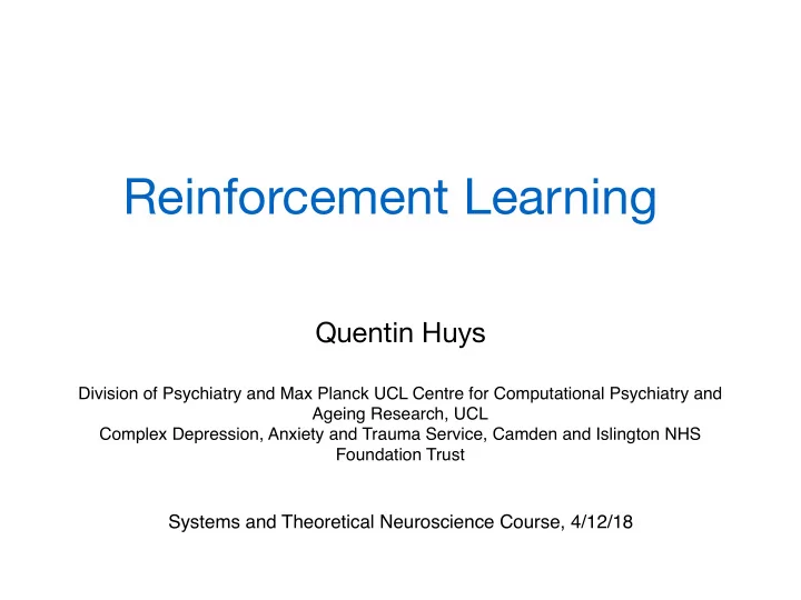
SLIDE 103

Quentin Huys RL SWC Ponel A,oversive excitor ponet B _ottroctivc inhibitor (Rescorlo, (Drckrnson, 1976 )

220 orcxrrusoN AND DEARTNG

9

F

< o.3

z

;

a O,z

U

&

c

l

' o.t

z

U

  • 8. APPETITIVE-AVERSIVE INTERACTIONS 221

reported a similar demonstration of the blocking of aversive conditioning by

an attractive inhibitor.

The implication of the transreinforcer blocking experiment is that an at- tractive inhibitor is functionally similar to an aversive excitor in its capacity

to modulate the aversive-reinforcement process. This parallel would, of

course, be strengthened if the similarity could be extended to other proper- ties of aversive excitors. Wagner (1971) reported an experiment in which it

was found, using a rabbit eyelid-conditioning preparation, that when two

excitors are presented in compound and nonreinforced, more extinction oc-

curred to one stimulus if the other was a strong rather than a weak excitor.

This enhancement of extinction can also be demonstrated in conditioned

suppression (Dickinson, 197Q. One group of rats, Group P, received the

light, A, paired with shock in the first stage and the tone, X, also paired

with shock in second stage, as in condition I of Table 8.5. These two aver-

sive excitors were then presented in compound and nonreinforced in a third

  • stage. Finally, the residual amount of conditioning to X was measured on

tone-alone test trials. Control groups received exactly the same training ex-

cept during the first stage. In this stage, the light, A, was associated with shock omission for the Group U, was semirandomly associated with shock

for Group R, and was not presented for Group no-CS. The enhancement of

aversive extinction is illustrated in Panel A of Fig. 8.7 by the fact that Group P showed less suppression to the tone, X, than the control groups on

the test trials. Enhancement of extinction can be explained in the same terms

as blocking, by assuming that the amount of extinction occurring to a CS is

a positive function of the level of arousal of the aversive system at the time the CS is presented (Konorski, 1948; Rescorla, 1973). Simultaneous presen-

tation of another aversive excitor just increases this level.

TABLE 8.5

Enhancement of aversive extinction ('onditions

Stage I Stoge 2 Stoge 3

R

NO.CS U

U R NO-CS P GROUPS

FIG' 8.6. Brocking of aversive condirioning: Mean suppression ratios to added ele-

ment x on test. Paner A: Blocking when A established as aversive excitor in Group p.

values estimated from graphic data presented by Rescorra (1971) for first session of

testing, Panel B.' Blocking when A established as attractive inhibitor in Group U. p: paired groups; U: unpaired groups; R; random groups; no_CS: no-CS groups.

returned and pressing reestablished. In stage 2 the light, A, was com_

pounded with a novel 300GHztone, X, and the compound paired with a 0.5-ma 0.5-sec shock for 6 trials. Finally the amount of suppiession condi- tioned to the tone was measured by presenting it alone on i-t"rt trials. The

control groups received exactly the same training except during the ap. petitive conditioning stage. All control animals expeiienced Ih, ,urn.

clicker-food pairings as Group U. The differences were that the light was

semirandomly associated with food for Group R, paired with food for

Group P, and not presented at all during this itage ior Group no-cs.

Panel B of Fig. 8.6 illustrates the suppression maintained by the tone, x,

  • n the test trials. The tone maintained less aversive conditioning or suppres-

sion in Group U, for whom the light, A, was estabrished as a-potentiar at- tractive inhibitor than in the control groups., An overall analysis of test sup

pression ratios showed that there was a significant differente between the groups (p ( o.os); and individual comparilns by the Newman-Keuls pro- cedure revealed that Group U was significantly less suppressed than both

Groups P and no-cS (p < 0.05 in both cases). Fowler (in press) has recentry

'lIt vicw 0l lltc Drcvitttts (lclll()rrslrirli()n llr:rl :ur :lltr;r('lrvt. crt.ilor (.()ul(l l)r(xllrr-(. \rrl)cl(.(r.

cliliorrirrg, orrt.rrrighl lr:rvc t.rpct.tt.tl lltc P:rrrcrl Ironl) to sltow rrrrrrt.\rrIl)t(.,,:,tolt lrr \ llriur tlrr.

{)lll('l l',1()lll)\ llt lltc l(.\l Arry rrrpr'l|orrltlr,,r;1111r. ltowr.\,r,1, wrtt Ir0lItlrlv

  • 1

r . , r 1 1 1 1 . , 1

1,r., "lkxl"

t.llt.r'l trt llrc 1r1r..,qs11 r.\lx.rnlr.nl

d+

5hscl(

control treatments

A+

food ommission

X- shock AX X* shock AX X+ shock AX

X

X X

In the next experiment, Dickinson (1976) attempted to find out whether

an attractive inhibitor would similarly enhance aversive extinction by com- paring conditions 2 and 3 of rable 8.5. Again after lever pressing had been

initially established, paired, unpaired, random, and no-CS groups were run,

rrsing cxactly the same classical appetitive conditioning schedules during

stagc I as cmploycd in thc transreinforcer blocking experiment. As a result,

tlrc light, A, should havt'bccorrrc an allractive inhibitor in Croup U.

'l'hcrcal'lcr, lhc prrrccdrlrc, lirllowcrl llral lor llrc crrhalrcclncnl ol' lhc

Value matters - transreinforcer blocking

Dickinson and Dearing 1979

218 orct<trlsoN AND DEARTNG

central system activated by an excitor. The alternative view (Konorski, 1967)

is that an excitatory association is formed between the CS representation

and some other central mechanism-an "antidrive" center or "no-LJS"

unit-whose arousal in turn leads to the inhibition of the excitatory system.

This is no place to go into Konorski's reasons for finally prefering the

second view, and for the present purposes it is only important to note that,

according to both models, the effect of an inhibitory stimulus is the

presence of an inhibitory influence on the relevant motivational system. Fig.

8.5 illustrates the path of such an influence for an attractive inhibitor, with

the question mark leaving open the actual associative structure of path.

In the absence of any excitatory influence on the appetitive and aversive

systems, presentation of an attractive inhibitor, for example, will be without

an effect. However, if both systems are under an excitatory influence, their

potential levels of arousal will be reduced by mutual inhibition. If we now

present an attractive inhibitor, the level of activity in the appetitive system

will be reduced and correspondingly the level of activity in the aversive

system increased. As far as the excitatory functions of the aversive system

are concerned, the presentation of an attractive inhibitor should be func-

tionally equivalent to that of an aversive excitor (see Fig. 8.5). What we now need is a procedure with which to test this prediction.

Kamin (1969) demonstrated that if a stimulus, A, was paired with shock

  • ve15r'/e excrtor
  • ttr6q1lv"

rnh,b tor

  • ttroctrve

excrtor

  • B. APPETITIVE-AVERSIVE INTERACTIONS 219

before aversive conditioning to a compound stimulus, AX, in a conditioned- suppression procedure, the amount of conditioning accruing to X was

reduced or blocked. (See conditions I and 2 of Table 8.4.) This

phenomenon of blocking can be illustrated by considering two further groups run by Rescorla (1971). In addition to groups receiving A, a tone, and shock unpaired (Group tI) and randomly related (Group R) in stage 1,

Rescorla also ran groups that received either A and shock paired to establish

A an an aversive excitor (Group P), or no preexposure to A (Group no-CS)

before aversive conditioning to the AX compound in stage 2. Panel A of

  • Fig. 8.6 illustrates the suppression maintained by X alone during the first

test session. Less aversive conditioning accrued to X in Group P (condition

I of Table 8.4) than in Group R and Group no-CS (condition 2 of Table

8.4). Blocking can be explained if it is assumed that the amount of condi- tioning to a CS is positively related to the difference between the level of

arousal of the aversive system when the shock is presented and during the

CS (Konorski, 1948; Rescorla, 1973). Presentation of the pretrained aversive

excitor, A, during conditioning to AX decreases this discrepancy, and hence the amount of conditioning to X.

TABLE 8.4

Blocking of aversive conditioning

Oonditions

Stage I Stage 2 test

  • FlG. 8.5. Illustralion ol thc cllccl ()l iur irttr:r(tivc irrlribitor orr llrt'opporrcnt l)l(x('ss

syslcrn un(lcr llrr coltctrrrcrrl irrlltrt.tttt.()l itllt;lrllvr irrrtl lrvtrsive cxeilor:. €

:

rx

cilltltlly (olur(li()n, l: irrlrilrrlory r'otlrr.r liorr: 'l rrrr,.pcr rlrul p;rllrs (sr'c lrxl); > > >'

Ittileti0tt:tllv cr;rrrv:rlt'rrl ('x( tlitlotv rrrllrrr.rrr r. (.,r.{. tr.\t)

A+

shock

control treatments

traf66d

  • mmission

AX..* shock AX-

shock

AX+ shock

X X X

In many ways this procedure provides an ideal way of testing the func-

tional equivalence of an aversive excitor and attractive inhibitor. If such an

equivalence exists, an attractive inhibitor should also be capable of blocking aversive conditioning by a shock. The presentation of both shock and food

during the conditioned-suppression procedure will ensure the concurrent

arousal of both the appetitive and aversive systems during presentation of the inhibitor. To test this prediction, Dickinson (1976) initially trained rats to lever press for food on a variable-interval schedule with a mean of 2 min.

'Ihe lever was then withdrawn and classical appetitive conditioning ad-

  • rninistered. Stimulus A, a 3Gsec overhead light, was established as a poten-

tial attractive inhibitor for Group U by associating it with the omission of

lood, as in stage I of condition 3 in Table 8.4. This was done by intermixing

prcsentation of a 30-sec clicker, during which free food was delivered on a variablc-timc schedule with a mean of 7.5 sec, with nonreinforced presenta- tions ol'a clickcr-light compound. Alter 8 sessions, each containing 5 rein- lirrcerl clickcr arrcl 5 rrorrrcirrlilrccd clickcr lighl prcscntalions, thc lcvcr was

\, .t

(,

\

  • -fr*-r-.-l
  • --]

syqt e m

l1

“bad” vs “good”

slide-104
SLIDE 104

Quentin Huys RL SWC

Signtracking

Flagel et al., 2011 Nature, Huys et al., 2014 Prog. Neurobiol.

Peak [DA] change (nM) Peak [DA] change (nM)

1 2 3 4 5 6 1 2 3 10 20 30 10 20 30 4 5 6

Session 1 Session 6 Session 1 Session 6 CS US CS US

Sign trackers Goal trackers

CS US Time CS US Time

A B C D E F

slide-105
SLIDE 105

Quentin Huys RL SWC

Signtracking

Flagel et al., 2011 Nature, Huys et al., 2014 Prog. Neurobiol.

Peak [DA] change (nM) Peak [DA] change (nM)

1 2 3 4 5 6 1 2 3 10 20 30 10 20 30 4 5 6

Session 1 Session 6 Session 1 Session 6 CS US CS US

Sign trackers Goal trackers

CS US Time CS US Time

A B C D E F

slide-106
SLIDE 106

Quentin Huys RL SWC

Absent model?

Flagel et al., 2011 Nature

c

Session 1 2 3 4 6 5 CS US 20 nM 20 s

e

CS US 20 nM Session 1 2 3 4 6 5 20 s

Sign trackers Goal trackers

δ = r − Q

slide-107
SLIDE 107

Quentin Huys RL SWC

Absent model?

Flagel et al., 2011 Nature

c

Session 1 2 3 4 6 5 CS US 20 nM 20 s

e

CS US 20 nM Session 1 2 3 4 6 5 20 s

a b

0.0 0.2 0.4 0.6 0.8 1.0 Probability 0.0 0.2 0.4 0.6 0.8 1.0 Sign-tracking bHR rats

d a

*

Goal-tracking bLR rats

Sign trackers Goal trackers

δ = r − Q

slide-108
SLIDE 108

Quentin Huys RL SWC

Sign-tracking in humans?

Schad et al., in prep

slide-109
SLIDE 109

Quentin Huys RL SWC

Sign-tracking in humans?

Schad et al., in prep

slide-110
SLIDE 110

Quentin Huys RL SWC

Double dissociation between ST and GT

Schad et al., in prep

slide-111
SLIDE 111

Quentin Huys RL SWC

Double dissociation between ST and GT

Schad et al., in prep

slide-112
SLIDE 112

Quentin Huys RL SWC

Goal-tracking in humans?

Schad et al., in prep

ST: learn expected value V GT: learn mappings T from CS to US identity

V(s) = X

a

π(a; s) X

s0

T (s0|s, a)[R(s0, a, s) + V(s0)]

slide-113
SLIDE 113

Quentin Huys RL SWC

Double dissociation between ST and GT

Schad et al., in prep

slide-114
SLIDE 114

Quentin Huys RL SWC

Successor representation

vπ = (I − Tπ)−1Rπ

V π(s) = X

a

π(a|s) X

s0

T a

ss0[Ra ss0 + V (s0)]

<latexit sha1_base64="AP7ecM067p75BsHwyhDvbuZ6AMg=">ACQXicbZBLSwMxFIUzvq2vqks3wSKdIsiMCLoRDcuq7S10JmWO2mhmYeJBmhjPX3PgP3Ll340IRt27MtMVH9UDg5Lv3kpvjxZxJZVmPxtT0zOzc/MJiYWl5ZXWtuL7RkFEiCK2TiEei6YGknIW0rpjitBkLCoH6ZXP8vrVzdUSBaFNTWIqRtAL2Q+I6A06hSbjXbqxCwzZQUfY0cmQSeFTBMTbmVldJflDsBqGsCPK1lbdAoZ60vePkNd3HDlOWK2ymWrD1rKPzX2GNTQmNVO8UHpxuRJKChIhykbNlWrNwUhGKE06zgJLGQPrQoy1tQwiodNhAhne0aSL/UjoEyo8pD8nUgikHASe7sx3lpO1HP5XayXKP3JTFsaJoiEZPeQnHKsI53HiLhOUKD7QBohgeldMrkEAUTr0g7BnvzyX9PY37O1vzgonZyO41hAW2gbmchGh+gEnaMqiOC7tATekGvxr3xbLwZ76PWKWM8s4l+yfj4BEoSsAo=</latexit><latexit sha1_base64="AP7ecM067p75BsHwyhDvbuZ6AMg=">ACQXicbZBLSwMxFIUzvq2vqks3wSKdIsiMCLoRDcuq7S10JmWO2mhmYeJBmhjPX3PgP3Ll340IRt27MtMVH9UDg5Lv3kpvjxZxJZVmPxtT0zOzc/MJiYWl5ZXWtuL7RkFEiCK2TiEei6YGknIW0rpjitBkLCoH6ZXP8vrVzdUSBaFNTWIqRtAL2Q+I6A06hSbjXbqxCwzZQUfY0cmQSeFTBMTbmVldJflDsBqGsCPK1lbdAoZ60vePkNd3HDlOWK2ymWrD1rKPzX2GNTQmNVO8UHpxuRJKChIhykbNlWrNwUhGKE06zgJLGQPrQoy1tQwiodNhAhne0aSL/UjoEyo8pD8nUgikHASe7sx3lpO1HP5XayXKP3JTFsaJoiEZPeQnHKsI53HiLhOUKD7QBohgeldMrkEAUTr0g7BnvzyX9PY37O1vzgonZyO41hAW2gbmchGh+gEnaMqiOC7tATekGvxr3xbLwZ76PWKWM8s4l+yfj4BEoSsAo=</latexit><latexit sha1_base64="AP7ecM067p75BsHwyhDvbuZ6AMg=">ACQXicbZBLSwMxFIUzvq2vqks3wSKdIsiMCLoRDcuq7S10JmWO2mhmYeJBmhjPX3PgP3Ll340IRt27MtMVH9UDg5Lv3kpvjxZxJZVmPxtT0zOzc/MJiYWl5ZXWtuL7RkFEiCK2TiEei6YGknIW0rpjitBkLCoH6ZXP8vrVzdUSBaFNTWIqRtAL2Q+I6A06hSbjXbqxCwzZQUfY0cmQSeFTBMTbmVldJflDsBqGsCPK1lbdAoZ60vePkNd3HDlOWK2ymWrD1rKPzX2GNTQmNVO8UHpxuRJKChIhykbNlWrNwUhGKE06zgJLGQPrQoy1tQwiodNhAhne0aSL/UjoEyo8pD8nUgikHASe7sx3lpO1HP5XayXKP3JTFsaJoiEZPeQnHKsI53HiLhOUKD7QBohgeldMrkEAUTr0g7BnvzyX9PY37O1vzgonZyO41hAW2gbmchGh+gEnaMqiOC7tATekGvxr3xbLwZ76PWKWM8s4l+yfj4BEoSsAo=</latexit><latexit sha1_base64="AP7ecM067p75BsHwyhDvbuZ6AMg=">ACQXicbZBLSwMxFIUzvq2vqks3wSKdIsiMCLoRDcuq7S10JmWO2mhmYeJBmhjPX3PgP3Ll340IRt27MtMVH9UDg5Lv3kpvjxZxJZVmPxtT0zOzc/MJiYWl5ZXWtuL7RkFEiCK2TiEei6YGknIW0rpjitBkLCoH6ZXP8vrVzdUSBaFNTWIqRtAL2Q+I6A06hSbjXbqxCwzZQUfY0cmQSeFTBMTbmVldJflDsBqGsCPK1lbdAoZ60vePkNd3HDlOWK2ymWrD1rKPzX2GNTQmNVO8UHpxuRJKChIhykbNlWrNwUhGKE06zgJLGQPrQoy1tQwiodNhAhne0aSL/UjoEyo8pD8nUgikHASe7sx3lpO1HP5XayXKP3JTFsaJoiEZPeQnHKsI53HiLhOUKD7QBohgeldMrkEAUTr0g7BnvzyX9PY37O1vzgonZyO41hAW2gbmchGh+gEnaMqiOC7tATekGvxr3xbLwZ76PWKWM8s4l+yfj4BEoSsAo=</latexit>

vπ = Rπ + Tπvπ

<latexit sha1_base64="VeWe0CkT5bUi978FZRPc7Ytfjo=">ACL3icbZBdS8MwFIZTP+f8qnrpTXAIgjBaEfRGAri5ZR9wVpHmqVbWJqWJB2M0n/kjX9lNyKeOu/MN060c0XAi/POYec83oRo1JZ1quxtLyurZe2Chubm3v7Jp7+w0ZxgKTOg5ZKFoekoRTuqKkZakSAo8BhpeoObrN4cEiFpyGtqFBE3QD1OfYqR0qhj3joBUn3PT4bpY+JENIVXcIYeZuj0B9VyND/VMUtW2ZoILho7NyWQq9ox043xHFAuMIMSdm2rUi5CRKYkbSohNLEiE8QD3S1pajgEg3mdybwmNutAPhX5cwQn9PZGgQMpR4OnObE85X8vgf7V2rPxLN6E8ihXhePqRHzOoQpiFB7tUEKzYSBuEBdW7QtxHAmGlIy7qEOz5kxdN46xsa39/Xqpc53EUwCE4AifABhegAu5AFdQBk9gDN7Au/FsvBgfxue0dcnIZw7AHxlf325qyU=</latexit><latexit sha1_base64="VeWe0CkT5bUi978FZRPc7Ytfjo=">ACL3icbZBdS8MwFIZTP+f8qnrpTXAIgjBaEfRGAri5ZR9wVpHmqVbWJqWJB2M0n/kjX9lNyKeOu/MN060c0XAi/POYec83oRo1JZ1quxtLyurZe2Chubm3v7Jp7+w0ZxgKTOg5ZKFoekoRTuqKkZakSAo8BhpeoObrN4cEiFpyGtqFBE3QD1OfYqR0qhj3joBUn3PT4bpY+JENIVXcIYeZuj0B9VyND/VMUtW2ZoILho7NyWQq9ox043xHFAuMIMSdm2rUi5CRKYkbSohNLEiE8QD3S1pajgEg3mdybwmNutAPhX5cwQn9PZGgQMpR4OnObE85X8vgf7V2rPxLN6E8ihXhePqRHzOoQpiFB7tUEKzYSBuEBdW7QtxHAmGlIy7qEOz5kxdN46xsa39/Xqpc53EUwCE4AifABhegAu5AFdQBk9gDN7Au/FsvBgfxue0dcnIZw7AHxlf325qyU=</latexit><latexit sha1_base64="VeWe0CkT5bUi978FZRPc7Ytfjo=">ACL3icbZBdS8MwFIZTP+f8qnrpTXAIgjBaEfRGAri5ZR9wVpHmqVbWJqWJB2M0n/kjX9lNyKeOu/MN060c0XAi/POYec83oRo1JZ1quxtLyurZe2Chubm3v7Jp7+w0ZxgKTOg5ZKFoekoRTuqKkZakSAo8BhpeoObrN4cEiFpyGtqFBE3QD1OfYqR0qhj3joBUn3PT4bpY+JENIVXcIYeZuj0B9VyND/VMUtW2ZoILho7NyWQq9ox043xHFAuMIMSdm2rUi5CRKYkbSohNLEiE8QD3S1pajgEg3mdybwmNutAPhX5cwQn9PZGgQMpR4OnObE85X8vgf7V2rPxLN6E8ihXhePqRHzOoQpiFB7tUEKzYSBuEBdW7QtxHAmGlIy7qEOz5kxdN46xsa39/Xqpc53EUwCE4AifABhegAu5AFdQBk9gDN7Au/FsvBgfxue0dcnIZw7AHxlf325qyU=</latexit><latexit sha1_base64="VeWe0CkT5bUi978FZRPc7Ytfjo=">ACL3icbZBdS8MwFIZTP+f8qnrpTXAIgjBaEfRGAri5ZR9wVpHmqVbWJqWJB2M0n/kjX9lNyKeOu/MN060c0XAi/POYec83oRo1JZ1quxtLyurZe2Chubm3v7Jp7+w0ZxgKTOg5ZKFoekoRTuqKkZakSAo8BhpeoObrN4cEiFpyGtqFBE3QD1OfYqR0qhj3joBUn3PT4bpY+JENIVXcIYeZuj0B9VyND/VMUtW2ZoILho7NyWQq9ox043xHFAuMIMSdm2rUi5CRKYkbSohNLEiE8QD3S1pajgEg3mdybwmNutAPhX5cwQn9PZGgQMpR4OnObE85X8vgf7V2rPxLN6E8ihXhePqRHzOoQpiFB7tUEKzYSBuEBdW7QtxHAmGlIy7qEOz5kxdN46xsa39/Xqpc53EUwCE4AifABhegAu5AFdQBk9gDN7Au/FsvBgfxue0dcnIZw7AHxlf325qyU=</latexit>

ˆ v = Mw

<latexit sha1_base64="W7BqrA7RDpHbJVJfvdlhpg+jCQg=">ACEHicbZBLS8NAEMc39VXrK+rRy2IRPZVEBL0IRS9ehAr2AW0om+2mXbp5sDuplJCP4MWv4sWDIl49evPbuGlT0NaBhd/+Z4aZ+buR4Aos69soLC2vrK4V10sbm1vbO+buXkOFsaSsTkMRypZLFBM8YHXgIFgrkoz4rmBNd3id5ZsjJhUPg3sYR8zxST/gHqcEtNQ1jzsDAknHJzBwvWSUpvgSz3636Ywe0q5ZtirWJPAi2DmUR61rvnV6YU09lkAVBCl2rYVgZMQCZwKlpY6sWIRoUPSZ2NAfGZcpLJQSk+0koPe6HULwA8UX93JMRXauy7ujLbUM3nMvG/XDsG78JeBDFwAI6HeTFAkOIM3dwj0tGQYw1ECq53hXTAZGEgvawpE2w509ehMZpxdZ8d1auXuV2FNEBOkQnyEbnqIpuUA3VEUWP6Bm9ojfjyXgx3o2PaWnByHv20Z8wPn8A9kOdyw=</latexit><latexit sha1_base64="W7BqrA7RDpHbJVJfvdlhpg+jCQg=">ACEHicbZBLS8NAEMc39VXrK+rRy2IRPZVEBL0IRS9ehAr2AW0om+2mXbp5sDuplJCP4MWv4sWDIl49evPbuGlT0NaBhd/+Z4aZ+buR4Aos69soLC2vrK4V10sbm1vbO+buXkOFsaSsTkMRypZLFBM8YHXgIFgrkoz4rmBNd3id5ZsjJhUPg3sYR8zxST/gHqcEtNQ1jzsDAknHJzBwvWSUpvgSz3636Ywe0q5ZtirWJPAi2DmUR61rvnV6YU09lkAVBCl2rYVgZMQCZwKlpY6sWIRoUPSZ2NAfGZcpLJQSk+0koPe6HULwA8UX93JMRXauy7ujLbUM3nMvG/XDsG78JeBDFwAI6HeTFAkOIM3dwj0tGQYw1ECq53hXTAZGEgvawpE2w509ehMZpxdZ8d1auXuV2FNEBOkQnyEbnqIpuUA3VEUWP6Bm9ojfjyXgx3o2PaWnByHv20Z8wPn8A9kOdyw=</latexit><latexit sha1_base64="W7BqrA7RDpHbJVJfvdlhpg+jCQg=">ACEHicbZBLS8NAEMc39VXrK+rRy2IRPZVEBL0IRS9ehAr2AW0om+2mXbp5sDuplJCP4MWv4sWDIl49evPbuGlT0NaBhd/+Z4aZ+buR4Aos69soLC2vrK4V10sbm1vbO+buXkOFsaSsTkMRypZLFBM8YHXgIFgrkoz4rmBNd3id5ZsjJhUPg3sYR8zxST/gHqcEtNQ1jzsDAknHJzBwvWSUpvgSz3636Ywe0q5ZtirWJPAi2DmUR61rvnV6YU09lkAVBCl2rYVgZMQCZwKlpY6sWIRoUPSZ2NAfGZcpLJQSk+0koPe6HULwA8UX93JMRXauy7ujLbUM3nMvG/XDsG78JeBDFwAI6HeTFAkOIM3dwj0tGQYw1ECq53hXTAZGEgvawpE2w509ehMZpxdZ8d1auXuV2FNEBOkQnyEbnqIpuUA3VEUWP6Bm9ojfjyXgx3o2PaWnByHv20Z8wPn8A9kOdyw=</latexit><latexit sha1_base64="W7BqrA7RDpHbJVJfvdlhpg+jCQg=">ACEHicbZBLS8NAEMc39VXrK+rRy2IRPZVEBL0IRS9ehAr2AW0om+2mXbp5sDuplJCP4MWv4sWDIl49evPbuGlT0NaBhd/+Z4aZ+buR4Aos69soLC2vrK4V10sbm1vbO+buXkOFsaSsTkMRypZLFBM8YHXgIFgrkoz4rmBNd3id5ZsjJhUPg3sYR8zxST/gHqcEtNQ1jzsDAknHJzBwvWSUpvgSz3636Ywe0q5ZtirWJPAi2DmUR61rvnV6YU09lkAVBCl2rYVgZMQCZwKlpY6sWIRoUPSZ2NAfGZcpLJQSk+0koPe6HULwA8UX93JMRXauy7ujLbUM3nMvG/XDsG78JeBDFwAI6HeTFAkOIM3dwj0tGQYw1ECq53hXTAZGEgvawpE2w509ehMZpxdZ8d1auXuV2FNEBOkQnyEbnqIpuUA3VEUWP6Bm9ojfjyXgx3o2PaWnByHv20Z8wPn8A9kOdyw=</latexit>
slide-115
SLIDE 115

Quentin Huys RL SWC

Learning a successor representation

Russek et al., 2017 PLoS Biol

Mpðs; :Þ ¼ 1s þ g P

s0Tpðs; s0ÞMpðs0; :Þ;

! MpÖs; :Ü MpÖs; :Ü á aSRâ1s á gMpÖs0; :Ü MpÖs; :Üä;

Mp à ÖI gTpÜ

1

slide-116
SLIDE 116

Quentin Huys RL SWC

Learning a successor representation

Russek et al., 2017 PLoS Biol

  • “Model-free learning”

Mpðs; :Þ ¼ 1s þ g P

s0Tpðs; s0ÞMpðs0; :Þ;

! MpÖs; :Ü MpÖs; :Ü á aSRâ1s á gMpÖs0; :Ü MpÖs; :Üä;

Mp à ÖI gTpÜ

1

slide-117
SLIDE 117

Quentin Huys RL SWC

Learning a successor representation

Russek et al., 2017 PLoS Biol

  • “Model-free learning”

Mpðs; :Þ ¼ 1s þ g P

s0Tpðs; s0ÞMpðs0; :Þ;

! MpÖs; :Ü MpÖs; :Ü á aSRâ1s á gMpÖs0; :Ü MpÖs; :Üä;

Mp à ÖI gTpÜ

1

slide-118
SLIDE 118

Quentin Huys RL SWC

Learning a successor representation

Russek et al., 2017 PLoS Biol

  • “Model-free learning”

Mpðs; :Þ ¼ 1s þ g P

s0Tpðs; s0ÞMpðs0; :Þ;

! MpÖs; :Ü MpÖs; :Ü á aSRâ1s á gMpÖs0; :Ü MpÖs; :Üä;

Mp à ÖI gTpÜ

1

slide-119
SLIDE 119

Quentin Huys RL SWC

Learning a successor representation

Russek et al., 2017 PLoS Biol

  • “Model-free learning”
  • “Model-based learning”
  • Estimate transition and compute

Mpðs; :Þ ¼ 1s þ g P

s0Tpðs; s0ÞMpðs0; :Þ;

! MpÖs; :Ü MpÖs; :Ü á aSRâ1s á gMpÖs0; :Ü MpÖs; :Üä;

Mp à ÖI gTpÜ

1

slide-120
SLIDE 120

Quentin Huys RL SWC

Learning a successor representation

Russek et al., 2017 PLoS Biol

  • “Model-free learning”
  • “Model-based learning”
  • Estimate transition and compute

Mpðs; :Þ ¼ 1s þ g P

s0Tpðs; s0ÞMpðs0; :Þ;

! MpÖs; :Ü MpÖs; :Ü á aSRâ1s á gMpÖs0; :Ü MpÖs; :Üä;

Mp à ÖI gTpÜ

1

slide-121
SLIDE 121

Quentin Huys RL SWC

Human successor learning

Momennejad et al., 2017 Nat. Hum. Beh.

$0 $15 $30 4 5 $0 $45 6 $30 $0 $15 $30 $15 $0 $30 $0 $15 $30 4 3 5 $0 $15 6 $30 4 5 $15 $45 6 $30 4 5 $0 $15 6 $45 2 4 3 5 6 1 2 4 3 5 6 1 2 4 3 5 6 1 2 4 3 5 6 1 2 1 1 1 1 Phase 1: learning Phase 2: re-learning Phase 3: test Reward revaluation Transition revaluation Policy revaluation Control

R e w a r d r e v a l u a t i
  • n
T r a n s i t i
  • n
r e v a l u a t i
  • n
P
  • l
i c y r e v a l u a t i
  • n
C
  • n
t r
  • l
0.2 0.4 0.6 0.8 Proportion of participants who changed preference
slide-122
SLIDE 122

Quentin Huys RL SWC

Human successor learning

Momennejad et al., 2017 Nat. Hum. Beh.

$0 $15 $30 4 5 $0 $45 6 $30 $0 $15 $30 $15 $0 $30 $0 $15 $30 4 3 5 $0 $15 6 $30 4 5 $15 $45 6 $30 4 5 $0 $15 6 $45 2 4 3 5 6 1 2 4 3 5 6 1 2 4 3 5 6 1 2 4 3 5 6 1 2 1 1 1 1 Phase 1: learning Phase 2: re-learning Phase 3: test Reward revaluation Transition revaluation Policy revaluation Control

R e w a r d r e v a l u a t i
  • n
T r a n s i t i
  • n
r e v a l u a t i
  • n
P
  • l
i c y r e v a l u a t i
  • n
C
  • n
t r
  • l
0.2 0.4 0.6 0.8 Proportion of participants who changed preference
slide-123
SLIDE 123

Quentin Huys RL SWC

Human successor learning

Momennejad et al., 2017 Nat. Hum. Beh.

$0 $15 $30 4 5 $0 $45 6 $30 $0 $15 $30 $15 $0 $30 $0 $15 $30 4 3 5 $0 $15 6 $30 4 5 $15 $45 6 $30 4 5 $0 $15 6 $45 2 4 3 5 6 1 2 4 3 5 6 1 2 4 3 5 6 1 2 4 3 5 6 1 2 1 1 1 1 Phase 1: learning Phase 2: re-learning Phase 3: test Reward revaluation Transition revaluation Policy revaluation Control

R e w a r d r e v a l u a t i
  • n
T r a n s i t i
  • n
r e v a l u a t i
  • n
P
  • l
i c y r e v a l u a t i
  • n
C
  • n
t r
  • l
0.2 0.4 0.6 0.8 Proportion of participants who changed preference
slide-124
SLIDE 124

Quentin Huys RL SWC

Human successor learning

Momennejad et al., 2017 Nat. Hum. Beh.

$0 $15 $30 4 5 $0 $45 6 $30 $0 $15 $30 $15 $0 $30 $0 $15 $30 4 3 5 $0 $15 6 $30 4 5 $15 $45 6 $30 4 5 $0 $15 6 $45 2 4 3 5 6 1 2 4 3 5 6 1 2 4 3 5 6 1 2 4 3 5 6 1 2 1 1 1 1 Phase 1: learning Phase 2: re-learning Phase 3: test Reward revaluation Transition revaluation Policy revaluation Control

R e w a r d r e v a l u a t i
  • n
T r a n s i t i
  • n
r e v a l u a t i
  • n
P
  • l
i c y r e v a l u a t i
  • n
C
  • n
t r
  • l
0.2 0.4 0.6 0.8 Proportion of participants who changed preference
slide-125
SLIDE 125

Quentin Huys RL SWC

Human successor learning

Momennejad et al., 2017 Nat. Hum. Beh.

$0 $15 $30 4 5 $0 $45 6 $30 $0 $15 $30 $15 $0 $30 $0 $15 $30 4 3 5 $0 $15 6 $30 4 5 $15 $45 6 $30 4 5 $0 $15 6 $45 2 4 3 5 6 1 2 4 3 5 6 1 2 4 3 5 6 1 2 4 3 5 6 1 2 1 1 1 1 Phase 1: learning Phase 2: re-learning Phase 3: test Reward revaluation Transition revaluation Policy revaluation Control

R e w a r d r e v a l u a t i
  • n
T r a n s i t i
  • n
r e v a l u a t i
  • n
P
  • l
i c y r e v a l u a t i
  • n
C
  • n
t r
  • l
0.2 0.4 0.6 0.8 Proportion of participants who changed preference
slide-126
SLIDE 126

Quentin Huys RL SWC

Human successor learning

Momennejad et al., 2017 Nat. Hum. Beh.

$0 $15 $30 4 5 $0 $45 6 $30 $0 $15 $30 $15 $0 $30 $0 $15 $30 4 3 5 $0 $15 6 $30 4 5 $15 $45 6 $30 4 5 $0 $15 6 $45 2 4 3 5 6 1 2 4 3 5 6 1 2 4 3 5 6 1 2 4 3 5 6 1 2 1 1 1 1 Phase 1: learning Phase 2: re-learning Phase 3: test Reward revaluation Transition revaluation Policy revaluation Control

R e w a r d r e v a l u a t i
  • n
T r a n s i t i
  • n
r e v a l u a t i
  • n
P
  • l
i c y r e v a l u a t i
  • n
C
  • n
t r
  • l
0.2 0.4 0.6 0.8 Proportion of participants who changed preference
slide-127
SLIDE 127

Quentin Huys RL SWC

Human successor learning

Momennejad et al., 2017 Nat. Hum. Beh.

$0 $15 $30 4 5 $0 $45 6 $30 $0 $15 $30 $15 $0 $30 $0 $15 $30 4 3 5 $0 $15 6 $30 4 5 $15 $45 6 $30 4 5 $0 $15 6 $45 2 4 3 5 6 1 2 4 3 5 6 1 2 4 3 5 6 1 2 4 3 5 6 1 2 1 1 1 1 Phase 1: learning Phase 2: re-learning Phase 3: test Reward revaluation Transition revaluation Policy revaluation Control

R e w a r d r e v a l u a t i
  • n
T r a n s i t i
  • n
r e v a l u a t i
  • n
P
  • l
i c y r e v a l u a t i
  • n
C
  • n
t r
  • l
0.2 0.4 0.6 0.8 Proportion of participants who changed preference