Reinforcement Learning You can think of supervised learning as the - - PDF document

SLIDE 1

1

Reinforcement learning: Markov Decision Processes

1

Reinforcement Learning

• You can think of supervised learning as the

teacher providing answers (the class labels)

• In reinforcement learning, the agent learns

based on a punishment/reward scheme

2

based on a punishment/reward scheme

• Before we can talk about reinforcement

learning, we need to introduce Markov Decision Processes

Decision Processes: General Description

• Decide what action to take next given that your

action will affect what happens in the future

• Real world examples:

– Robot path planning

3

– Elevator scheduling – Travel route planning – Aircraft navigation – Manufacturing processes – Network switching and routing

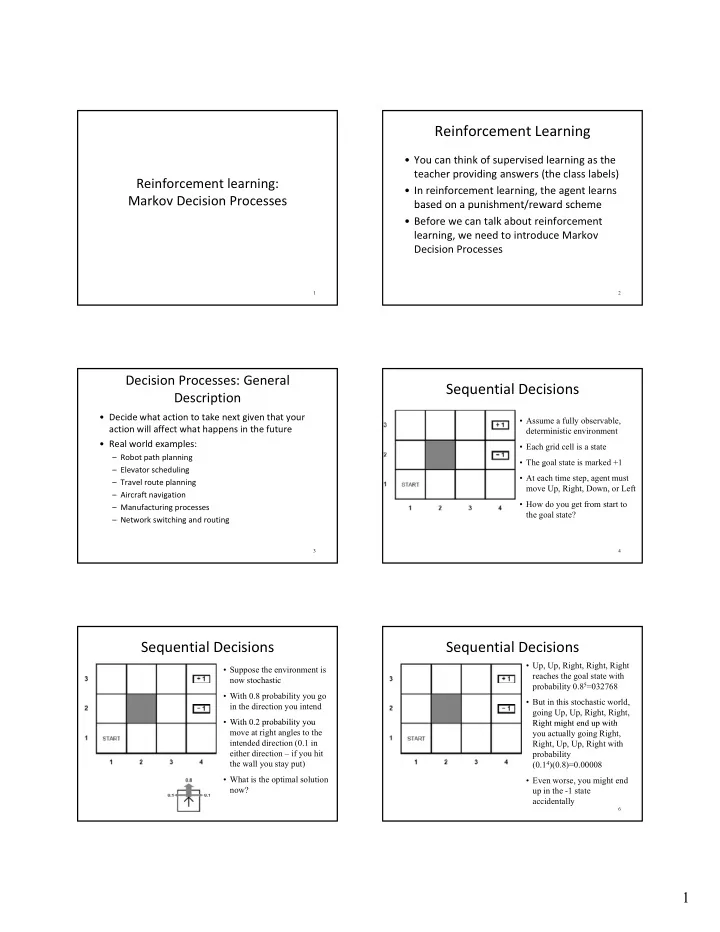
Sequential Decisions

• Assume a fully observable,

deterministic environment

• Each grid cell is a state
• The goal state is marked +1

4

g

• At each time step, agent must

move Up, Right, Down, or Left

• How do you get from start to

the goal state?

Sequential Decisions

• Suppose the environment is

now stochastic

• With 0.8 probability you go

in the direction you intend

• With 0 2 probability you

With 0.2 probability you move at right angles to the intended direction (0.1 in either direction – if you hit the wall you stay put)

• What is the optimal solution

now?

Sequential Decisions

• Up, Up, Right, Right, Right

reaches the goal state with probability 0.85=032768

• But in this stochastic world,

going Up, Up, Right, Right, Right might end up with

6

Right might end up with you actually going Right, Right, Up, Up, Right with probability (0.14)(0.8)=0.00008

• Even worse, you might end

up in the -1 state accidentally

SLIDE 2

2

Transition Model

• Transition model: a specification of the outcome

probabilities for each action in each possible state

• T(s, a, s’) = probability of going to state s’ if you are in

state s and do action a

• The transitions are Markovian ie. the probability of

reaching state s’ from s depends only on s and not on the

7

reaching state s from s depends only on s and not on the history of earlier states (aka The Markov Property)

• Mathematically:

Suppose you visited the following states in chronological

• rder: s0, …, st

P(st+1 | a, s0, …, st ) = P(st+1 | a, st)

Markov Property Example

Suppose s0 = (1,1), s1 = (1,2), s2 = (1,3) If I go right from state s2, the s s1 s2 s3

8

2

probability of going to s3 only depends on the fact that I am at state s2 and not the entire state history {s0, s1, s2} s0

The Reward Function

• Depends on the sequence of states (known

as the environment history)

• At each state s, the agent receives a reward

R(s) which may be positive or negative (but

9

R(s) which may be positive or negative (but must be bounded)

• For now, we’ll define the utility of an

environment history as the sum of the rewards received

Utility Function Example

R(4,3) = +1 (Agent wants to get here) R(4,2) = ‐1 (Agent wants to avoid this R(s) = ‐0.04 (for all other states) U(s1, …, sn) = R(s1) + … + R(sn)

10

If the states an agent goes through are Up, Up, Right, Right, Right, the utility of this environment history is:

• 0.04-0.04-0.04-0.04-0.04+1

Utility Function Example

If there’s no uncertainty, then the agent would find the sequence of actions that maximizes the sum of the rewards of the visited states

11

Markov Decision Process

The specification of a sequential decision problem for a fully observable environment with a Markovian transition model and additive rewards is called a Markov Decision Process (MDP) A MDP h th f ll i t

12

An MDP has the following components:

• 1. A finite set of states S along with an initial state

S0

• 2. A finite set of actions A
• 3. Transition Model: T(s, a, s’) = P( s’ | a, s )
• 4. Reward Function: R(s)

SLIDE 3

3

Solutions to an MDP

• Why is the following not a satisfactory

solution to the MDP?

[1,1]‐Up [1,2]‐Up

13

[ , ] p [1,3]‐Right [2,3]‐Right [3,3]‐Right

A Policy

• Policy: mapping from a state to an action
• Need this to be defined for all states so

that the agent will always know what to do

• Notation:

14

• Notation:

– π denotes a policy – π(s) denotes the action recommended by the policy π for state s

Optimal Policy

• There are obviously many different policies for an MDP
• Some are better than others. The “best” one is called the
• ptimal policy π* (we will define best more precisely in

later slides)

• Note: every time we start at the initial state and execute a

policy we get a different environment history (due to the

15

policy, we get a different environment history (due to the stochastic nature of the environment)

• This means we get a different utility every time we

execute a policy

• Need to measure expected utility ie. the average of the

utilities of the possible environment histories generated by the policy

Optimal Policy Example

R(s)=-0.04

16

Notice the tradeoff between risk and reward!

Roadmap for the Next Few Slides

We need to describe how to compute

• ptimal policies
• 1. Before we can do that, we need to define

the utility of a state

17

the utility of a state

• 2. Before we can do (1), we need to explain

stationarity assumption

• 3. Before we can do (2), we need to explain

finite/infinite horizons

Finite/Infinite Horizons

• Finite horizon: fixed time N after which nothing

matters (think of this as a deadline)

• Suppose our agent starts at (3,1), R(s)=‐0.04, and

N=3. Then to get to the +1 state, agent must go up. If N 100 t t k th f t d

18

• If N=100, agent can take the safe route around

SLIDE 4

4

Nonstationary Policies

• Nonstationary policy: the optimal action in a

given state changes over time

• With a finite horizon, the optimal policy is

nonstationary

• With an infinite horizon there is no incentive to

19

• With an infinite horizon, there is no incentive to

behave differently in the same state at different times

• With an infinite horizon, the optimal policy is

stationary

• We will assume infinite horizons

Utility of a State Sequence

Under stationarity, there are two ways to assign utilities to sequences: 1. Additive rewards: The utility of a state sequence is:

20

U(s0, s1, s2, …) = R(s0) + R(s1) + R(s2) + … 2. Discounted rewards: The utility of a state sequence is: U(s0, s1, s2, …) = R(s0) + γR(s1) + γ2R(s2) + … Where 0 ≤ γ ≤ 1 is the discount factor

The Discount Factor

• Describes preference for current rewards over

future rewards

• Compensates for uncertainty in available time

(models mortality)

• Eg Being promised $10000 next year is only

21

• Eg. Being promised $10000 next year is only

worth 90% of being promised $10000 now

• γ near 0 means future rewards don’t mean

anything

• γ = 1 makes discounted rewards equivalent to

additive rewards

Utilities

We assume infinite horizons. This means that if the agent doesn’t get to a terminal state, then environmental histories are infinite, and utilities with additive rewards are infinite. How do we deal with this? Discounted rewards makes utility finite. A i l t ibl d i R d 1

22

Assuming largest possible reward is Rmax and γ < 1, ) 1 ( ) ( ,...) , , (

max max 2 1

γ γ γ − = ≤ =

∑ ∑

∞ = ∞ =

R R s R s s s U

t t t t t

Computing Optimal Policies

• A policy π generates a sequence of states
• But the world is stochastic, so a policy π has

a range of possible state sequences, each

• f which has some probability of occurring

23

• f which has some probability of occurring
• The value of a policy is the expected sum of

discounted rewards obtained

The Optimal Policy

• Given a policy π, we write the expected

sum of discounted rewards obtained as:

⎥ ⎦ ⎤ ⎢ ⎣ ⎡∑

∞

| ) (

t t t

s R E π γ

24

⎦ ⎣ =0

t

• An optimal policy π* is the policy that

maximizes the expected sum above

⎥ ⎦ ⎤ ⎢ ⎣ ⎡ =

∑

∞ =0 *

| ) ( max arg

t t t

s R E π γ π

π

SLIDE 5

5

The Optimal Policy

• For every MDP, there exists an optimal policy
• There is no better option (in terms of expected

sum of rewards) than to follow this policy

• How do you calculate this optimal policy? Can’t

25

evaluate all policies…too many of them

• First, need to calculate the utility of each state
• Then use the state utilities to select an optimal

action in each state

Rewards vs Utilities

• What’s the difference between R(s) the

reward for a state and U(s) the utility of a state?

– R(s) – the short term reward for being in s

26

( ) g – U(s) – The long‐term total expected reward for the sequence of states starting at s (not just the reward for state s)

Utilities in the Maze Example

Start at state (1,1). Let’s suppose we choose the action Up.

27

U(1,1) = R(1,1) + ...

Reward for current state

Utilities in the Maze Example

Start at state (1,1). Let’s choose the action Up. U(1,1) = R(1,1) + 0.8*U(1,2) + 0.1*U(2,1) + 0.1*U(1,1)

Prob of moving up Prob of moving right Prob of moving left (into the wall) and staying put

Utilities in the Maze Example

Now let’s throw in the

29

discounting factor U(1,1) = R(1,1) + γ*0.8*U(1,2) + γ*0.1*U(2,1) +

γ*0.1*U(1,1)

The Utility of a State

∑

+ =

'

) ' ( ) ' , , ( ) ( ) (

s

s U s a s T s R s U γ

If we choose action a at state s, expected future rewards (discounted) are:

Reward at current state s Probability of moving from state s to state s’ by doing action a Expected sum of future discounted rewards starting at state s’ Expected sum of future discounted rewards starting at state s

SLIDE 6

6

The Utility of a State

• In the previous example, we chose the action a then

determined the utility of the state.

• The utility is really defined in terms of the optimal

action.

31

∑

+ =

'

) ' ( ) ' , , ( max ) ( ) (

s a

s U s a s T s R s U γ

• We modify the previous formula slightly by adding

a max term over actions.

The Utility of a State

∑

+ ) ' ( ) ' ( max ) ( ) ( s U s a s T s R s U γ

The utility of a state is the immediate reward for that state plus the expected discounted utility of the next state, assuming the agent chooses the optimal action

32

∑

+ =

'

) ' ( ) ' , , ( max ) ( ) (

s a

s U s a s T s R s U γ

This is the famous Bellman Equation

The Optimal Policy

• Selection of the action π*(s) = a which

maximizes the expected utility U(s)

• Intuitively, π* gives us the best action we

can take from any state to maximize our

33

can take from any state to maximize our future discounted rewards

∑

=

' *

) ' ( ) ' , , ( max arg ) (

s a

s U s a s T s π

What You Should Know

• How to formulate a problem as an MDP
• What the Markov property is
• How to calculate the utility for a state in an

MDP

34

MDP

• What the Bellman equation is