Regression L2: Curve fitting and Given a set of observations: x = { - - PDF document

L2: Curve fitting and probability theory

EECS 545: Machine Learning Benjamin Kuipers Winter 2009

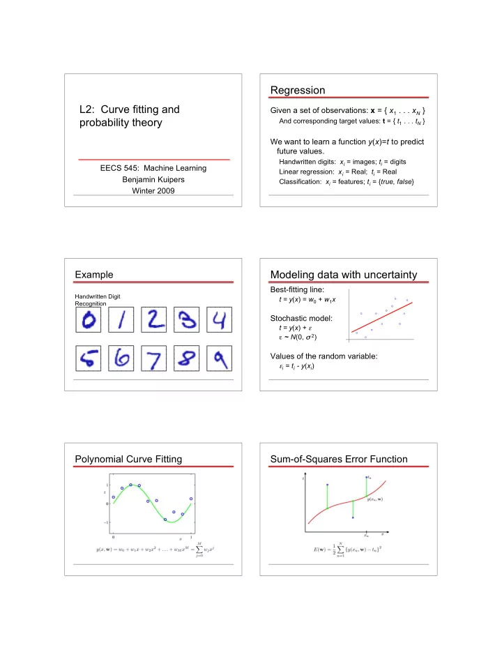
Regression

Given a set of observations: x = { x1 . . . xN }

And corresponding target values: t = { t1 . . . tN }

We want to learn a function y(x)=t to predict future values.

Handwritten digits: xi = images; ti = digits Linear regression: xi = Real; ti = Real Classification: xi = features; ti = {true, false}

Example

Handwritten Digit Recognition

Modeling data with uncertainty

Best-fitting line:

t = y(x) = w0 + w1x

Stochastic model:

t = y(x) + ε ε ~ N(0, σ 2)

Values of the random variable:

εi = ti - y(xi)

Polynomial Curve Fitting Sum-of-Squares Error Function

0th Order Polynomial 1st Order Polynomial 3rd Order Polynomial 9th Order Polynomial Over-fitting

Root-Mean-Square (RMS) Error:

Polynomial Coefficients

Data Set Size:

9th Order Polynomial

Data Set Size:

9th Order Polynomial

Regularization

Penalize large coefficient values

Regularization: Regularization: Regularization: vs.

Polynomial Coefficients

Where do we want to go?

We want to know our level of certainty. To do that, we need probability theory.

Probability Theory

Apples and Oranges

Probability Theory

Marginal Probability Conditional Probability Joint Probability

Probability Theory

Sum Rule Product Rule

The Rules of Probability

Sum Rule Product Rule

Bayes’ Theorem

posterior ∝ likelihood × prior

Probability Densities Transformed Densities Expectations

Conditional Expectation (discrete) Approximate Expectation (discrete and continuous)

Variances and Covariances

But what are probabilities?

This is a deep philosophical question!

Frequentists: Probabilities are frequencies of

• utcomes, over repeated experiments.

Bayesians: Probabilities are expressions of degrees of belief.

There’s only one consistent set of axioms.

But the two interpretations lead to very different ways to reason with probabilities.

Bayes’ Theorem

posterior ∝ likelihood × prior

The Gaussian Distribution Gaussian Mean and Variance The Multivariate Gaussian Gaussian Parameter Estimation

Likelihood function

Maximum (Log) Likelihood

Curve Fitting Re-visited Maximum Likelihood

Determine by minimizing sum-of-squares error, .

Predictive Distribution

MAP: A Step towards Bayes

Specify a prior distribution p(w|α) over the weight vector w. Gaussian with mean = 0, covariance = α -1I. Now compute posterior = likelihood * prior:

MAP: A Step towards Bayes

Determine by minimizing regularized sum-of-squares error, .

Where have we gotten, so far?

Least-squares curve fitting is equivalent to

Maximum likelihood parameter values, assuming Gaussian noise distribution.

Regularization is equivalent to

Maximum posterior parameter values, assuming Gaussian prior on parameters.

Fully Bayesian curve fitting introduces new ideas (wait for Section 3.3).

Bayesian Curve Fitting Bayesian Predictive Distribution

Next

The Curse of Dimensionality Decision Theory Information Theory