Reconstructing a Fragmented Face from a Cryptographic Identification - - PDF document

Reconstructing a Fragmented Face from a Cryptographic Identification Protocol

Andy Luong, Michael Gerbush, Brent Waters, Kristen Grauman Department of Computer Science, The University of Texas at Austin

aluong,mgerbush,bwaters,grauman@cs.utexas.edu

Abstract

Secure Computation of Face Identification (SCiFI) [20] is a recently developed secure face recognition system that ensures the list of faces it can identify (e.g., a terrorist watch list) remains private. In this work, we study the conse- quences of malformed input attacks on the system—from both a security and computer vision standpoint. In par- ticular, we present 1) a cryptographic attack that allows a dishonest user to undetectably obtain a coded represen- tation of faces on the list, and 2) a visualization approach that exploits this breach, turning the lossy recovered codes into human-identifiable face sketches. We evaluate our ap- proach on two challenging datasets, with face identification tasks given to a computer and human subjects. Whereas prior work considered security in the setting of honest in- puts and protocol execution, the success of our approach underscores the risk posed by malicious adversaries to to- days automatic face recognition systems.

• 1. Introduction

Face recognition research has tremendous implications for surveillance and security, and in recent years the field has seen much progress in terms of representations, learning algorithms, and challenging new datasets [31, 22]. At the same time, automatic systems to recognize faces (and other biometrics) naturally raise privacy concerns. Not only do individuals captured in surveillance images sacrifice some privacy about their activities, but system implementation choices can also jeopardize privacy—for example, if the list

• f persons of interest on a face recognition system ought to

remain confidential, but the system stores image exemplars. Recent work in security and computer vision explores how to simultaneously meet the privacy, efficiency, and ro- bustness requirements in such problems [28]. While se- cure facial matching is theoretically feasible by combining any recognition algorithm with general techniques for se- cure computation [30, 11], these methods are typically too slow to be deployed in real-time. Thus, researchers have

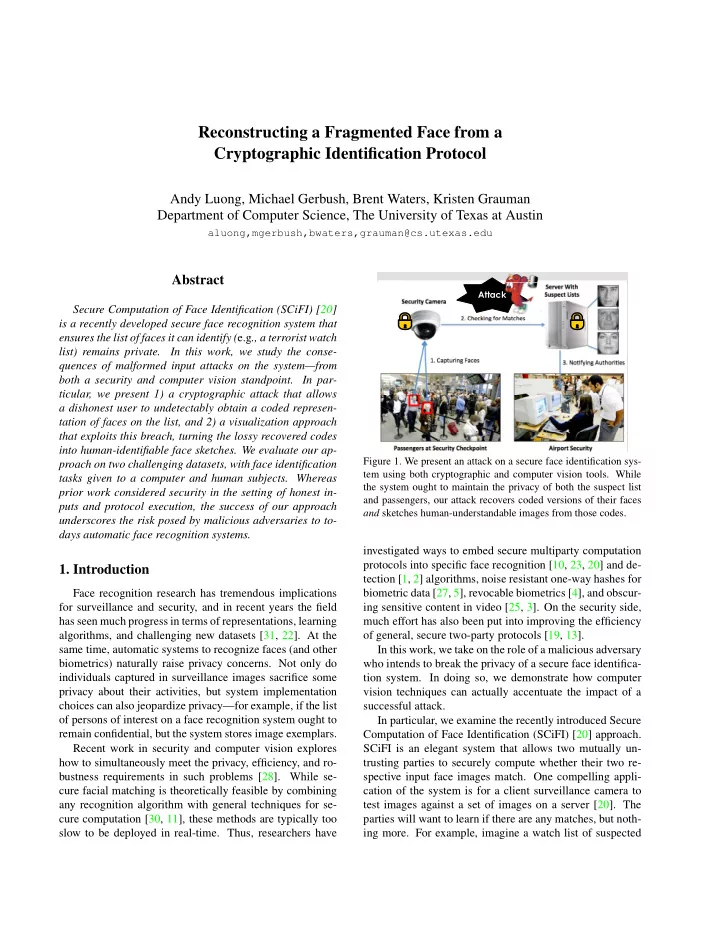
Attack

Figure 1. We present an attack on a secure face identification sys- tem using both cryptographic and computer vision tools. While the system ought to maintain the privacy of both the suspect list and passengers, our attack recovers coded versions of their faces and sketches human-understandable images from those codes.

investigated ways to embed secure multiparty computation protocols into specific face recognition [10, 23, 20] and de- tection [1, 2] algorithms, noise resistant one-way hashes for biometric data [27, 5], revocable biometrics [4], and obscur- ing sensitive content in video [25, 3]. On the security side, much effort has also been put into improving the efficiency

• f general, secure two-party protocols [19, 13].

In this work, we take on the role of a malicious adversary who intends to break the privacy of a secure face identifica- tion system. In doing so, we demonstrate how computer vision techniques can actually accentuate the impact of a successful attack. In particular, we examine the recently introduced Secure Computation of Face Identification (SCiFI) [20] approach. SCiFI is an elegant system that allows two mutually un- trusting parties to securely compute whether their two re- spective input face images match. One compelling appli- cation of the system is for a client surveillance camera to test images against a set of images on a server [20]. The parties will want to learn if there are any matches, but noth- ing more. For example, imagine a watch list of suspected

terrorists for an airport security system: the airport author- ities should be able to submit face images of passengers as queries, and learn only if they are on the list or not. How- ever, no one should be able to find out which individuals are on the list, nor should the database authority be able to create travel profiles of innocent parties. See Figure 1. The SCiFI protocol meets the desired properties under the “honest-but-curious” model of security [20], where security is guaranteed if each party follows the protocol. We investigate the consequences of a dishonest user that uses malformed inputs to attack the SCiFI protocol.1 Our work consists of two phases: a cryptographic attack phase and a visualization phase. For the first phase, we show that by submitting an ill-formed input, an attacker can learn if a particular feature is present in a target image. By repeating this attack multiple times, an entire vector encoding the fa- cial parts’ appearance and layout of a target person can be

• recovered. While recovering the facial vector alone consti-

tutes an attack, it is not necessarily usable by a human ob- server, since the result is a sparse set of patches with coarse

• layout. Thus, in the second phase, we show how to recon-

struct an image of the underlying face via computer vision

• techniques. Specifically, we draw on ideas in subspace anal-

ysis [9, 16, 24, 12, 29] to infer parts of the face not explicitly available in the recovered facial encoding. The resulting im- age is roughly comparable to a police sketch of a suspect, visualizing the identity our attack discovered. We evaluate our approach on two challenging datasets. We present qualitative examples of the visualized faces, and then quantify their quality based on identification tests for both human subjects and an automatic recognition sys-

• tem. Notably, we show that face images inferred by our

approach more closely resemble the true original faces than what could be visualized using data from the security break alone—illustrating how vision techniques can actually fa- cilitate attacks on a privacy-preserving system. Roadmap We first give necessary background for the SCiFI approach (Sec. 2). Then, we present our crypto- graphic attack (Sec. 3) and our associated face reconstruc- tion approach (Sec. 4). Finally, we present results in Sec. 5. We keep our explanation of our security contributions quite brief, in order to devote more space to the vision side. Please see the supplementary file2 for more details.

1We stress that our results do not contradict the claims of the origi-

nal SCiFI paper, which only claimed security in the setting of honest in- puts and protocol execution. Our attack therefore stretches the honest-but- curious constraints assumed in [20]. However, we believe it is important to consider: in real applications parties may be sufficiently motivated to launch malformed input attacks on such a system. Further, even if assum- ing benign parties, one party’s machine may be corrupted by an attacker who could then leverage the participant’s position to corrupt the system.

2http://vision.cs.utexas.edu/projects/securefaces

• 2. Background: The SCiFI System

First, we briefly overview the SCiFI system [20]. The server’s input is a list of faces, and the client’s input is a sin- gle face. The goal is to securely test whether the face input by the client is present in the server’s list, while allowing robustness in the matching. To this end, SCiFI develops a part-based face representation, a robust distance to compare two faces, and a secure client-server protocol to check for a match according to that distance, as we explain next. Face Representation Given a public database Y of face images, a standard set of p facial parts is extracted from each image (e.g., corners of the nose, mouth, eyes). For the i-th part, the system quantizes the associated image patches in Y to establish an appearance vocabulary V i = {V i

1 , . . . , V i N}

comprised of N prototypical examples (“visual words”) for that part. Note there are p such vocabularies. In ad- dition, each part has a corresponding spatial vocabulary Di = {Di

1, . . . , Di Q} consisting of Q quantized distances

• f the feature from the center of the face.

For some input face, let the set of its part patches be {I1, . . . , Ip}. For each Ii, two things are recorded. The first is the appearance component, and it contains the indices of the n visual words in V i that are most similar to the patch

• Ii. Denote this set sa

i ✓ {1, . . . , N}. The second part is

the spatial component, and it contains the indices of the z “distance words” in Di that are closest to Ii’s distance from the center of the face. Denote this set ss

i ✓ {1, . . . , Q}.

Combining all p such sets, the full face representation has the form ({sa

1, . . . , sa p}, {ss 1, . . . , ss p}).

Comparing Faces To compare two faces, SCiFI uses the symmetric difference between their two respective sets— that is, the number of elements which are in either of the sets and not in their intersection. The distance is computed separately for the appearance and spatial components, and then summed. If the total distance is under a given thresh-

• ld, the two faces are considered a match.

As shown in [20], the set difference is equivalent to the Hamming distance if the sets are each coded as l = p(N +Q)-bit binary vectors. Specifically, each set sa

i is rep-

resented by wa

i , an N-bit binary indicator vector for which

n entries are 1 (i.e., those n indices that are in sa

i ). Simi-

larly, each set ss

i is represented by ws i , a Q-bit binary indi-

cator vector for which z entries are 1. Then, the full repre- sentation for a given face is the concatenation of all these vectors: w = [wa

1, . . . , wa p, ws 1, . . . , ws p]. In the following

we refer to such a vector as a “face vector” or “facial code”. This conversion is valuable because the Hamming distance can be computed securely using cryptographic algorithms, as we briefly review next. Secure Protocol The input to the SCiFI protocol is a sin- gle face vector w from the client and a list of M face vectors

w1, . . . , wM and thresholds t1, . . . , tM from the server. Let H denote the Hamming distance. The output of the protocol is “match”, if H(wi, w) < ti for some i, and “no match”

• therwise.

The client uses an additively homomorphic encryption system [21]. The client shares the public key with the server and keeps the private key to itself. Encryption is done over Zm for some m = rq, where r and q are primes, while exploiting an exclusive-or implementation of the Hamming

• distance. Once the client has decrypted the server’s mes-

sage, an oblivious transfer protocol [18] is initiated. In short, both the client and server learn only if the Hamming distance between any pair of their vectors exceeds a thresh-

• ld. See [20] for details, including novel optimizations that

improve the efficiency.

• 3. Cryptographic Malformed Input Attack

The proposed attack on SCiFI allows the attacker to ob- tain a face code (w) that was meant to remain private. The attack relies on the fact that a dishonest adversary is able to input vectors of any form, not just vectors that are properly formatted.1 The attack learns the client’s face code bit-by- bit through the output of “match” or “no match”. Suppose the client’s vector is w. A dishonest server can add any vector wm to its suspect list, and choose each cor- responding threshold value, tm, arbitrarily. First, the server inputs the vector wm = [1, 0, . . . , 0], with a 1 in the first position and zero everywhere else. Next, the protocol com- paring w and wm is run as usual. By learning whether a match was detected, the server actually learns information about the first bit, w1, of the client’s input. We know that the nonzero entries of the input client vector must sum to exactly p(n+z). This creates two distinct possibilities in the outcome of the protocol:

• w1 = 1: In this case, the two input vectors will not dif-

fer in the first position. Therefore, they will only differ in the remaining p(n + z) 1 positions where w is

• nonzero. Hence, we know that the Hamming distance

between the two vectors is H(w, wm) = p(n+z)1.

• w1 = 0: In this case, the two input vectors will differ

in the first position. In addition, they will differ in all

• f the p(n + z) remaining places where w is nonzero.

Hence, we know the H(w, wm) = p(n + z) + 1. Taking advantage of these two possible outcomes, the dishonest server can fix the threshold tm = p(n+z). Then, if a match is found, it must be the case that H(w, wm) = p(n + z) 1  p(n + z), so w1 = 1. If a match is not found, then H(w, wm) = p(n + z) + 1 > p(n + z), so w1 = 0. Thus, the dishonest server can learn the first bit of the client’s input. Consequently, the attacker can learn the client’s entire vector by creating l vectors wi

m, 1  i  l,

where the i-th bit is set to 1. We have portrayed the attack from the perspective of the

Patch face Full face Figure 2. We first reconstruct the quantized patches based on the binary encoding (left), and then expand the reconstruction to hal- lucinate the full face given those patches (right).

server, where the server recovers facial codes for the client. However, we can also adapt this attack for the client, in which case the client learns the confidential faces on the

• server. See the supplementary file for details, as well as al-

gorithmic improvements that exploit the sparsity of the face representation to improve efficiency from O(p(N + Q)) to O(p(n log N + z log Q)).

• 4. Facial Reconstruction Approach

The cryptographic attack yields a binary vector encoding the appearance of some individual. However, the code itself is lossy compared to the original image, and spatially it cov- ers only about 40% of the face. Thus, we next propose an approach to form a human-interpretable visualization from the recovered binary encoding. The main idea is to first use the recovered indices of the most similar prototypical patches and spatial information for each facial part to render patches from the public vocab- ulary, placing each one according to the recovered approx- imate relative distance. This yields a “patch face” that fo- cuses on the key facial features (Sec. 4.2). Given this patch face, we then estimate a full face image using a subspace re- construction approach (Sec. 4.3). This “hallucinated face” integrates both the backprojected patches obtained from the attack as well as the learned statistics of faces in general. Figure 2 illustrates the two forms of reconstruction.

4.1. Offline Vocabulary and Subspace Learning

Before reconstructing any face, we must first perform two offline steps: (1) prepare the facial fragment “vocab- ularies”, and (2) construct a generic face subspace. As in the original SCiFI system, the face images used to create the vocabularies come from an external (possibly public) database Y , which can be completely unrelated to the people enrolled in the recognition system. All faces are normalized to a canonical scale, and the positions of key landmark features (i.e., corners of the eyes) are aligned. Given these face images, we use an unsupervised clus- tering algorithm (k-means) to quantize image patches and distances to form the appearance and spatial vocabularies

V 1, . . . , V p and D1, . . . , Dp (see Sec. 2). We also save a set

• f p unit displacement or “offset” vectors relative to the face

center, O = {o1, . . . , op}. For each face in Y , we extract the 2-D vector from the image center position to that in- stance’s i-th facial part, and then average all such vectors to

• btain oi. Note, the offset vectors are not in the SCiFI rep-

resentation; we will use them to estimate the placement of each reconstructed patch, in conjunction with the distance vocabulary indices coming from the recovered facial vec- tor. We also use Y to construct a generic face subspace. As has been long known in the face recognition com- munity [26, 17], the space of all face images occupies a lower-dimensional subspace within the space of all images. This fact can be exploited to compute low-dimensional image representations. While often used to perform nearest-neighbor face recognition (e.g., the Eigenface ap- proach [26]), we instead aim to exploit a face subspace in

• rder to “hallucinate” the portions of a reconstructed face

not covered by any of the p patches. Formally, let the face images in Y consist of a set of F vectors y0

1, . . . , y0 F , where each y0 i is formed by concate-

nating the pixel intensities in each row of the i-th image. We first compute the mean face µ =

1 F

PF

i=1 y0 i, and then

center the original faces by subtracting the mean from each

• ne. Let the matrix Y contain those centered face instances,

where each column is an instance: Y = [y1, . . . , yF ] = [y0

1 µ, . . . , y0 F µ].

Principal component analysis (PCA) identifies an or- dered set of F orthonormal vectors u1, . . . , uF that best describe the data, by capturing the directions with maxi- mal variance. By this definition, the desired vectors are the eigenvectors of the covariance matrix computed on Y , that is, the eigenvectors of

1 F

PF

i=1 yiyT i

= Y Y T , sorted by the magnitude of their associated eigenvalues. The top K eigenvectors define a K-dimensional face subspace. At this point, we have the part vocabularies V 1, . . . , V p, the distance vocabularies D1, . . . , Dp, and the displacement vectors O (all of which we will use to compute patch faces), and a face subspace defined by u1 . . . , uK (which we will use to compute full face reconstructions).

4.2. Patch Face Reconstruction

Now we can define the “patch face” reconstruction pro-

• cess. The cryptographic attack defined above yields the n

selected appearance vocabulary words and z selected dis- tance words, for each of the p facial parts. This encoding specifies the indices into the public vocabularies, revealing which prototypical appearances (and distances) were most similar to those that occurred in the original face. Thus, we retrieve the corresponding quantized patches and distance values for each part, and map them into an image buffer. To reconstruct the appearance of a part i, we take the n quantized patches and simply average them, since the code does not reveal which among the n was the

• closest. We place the resulting average into the buffer rel-

ative to its center, displaced according to the direction oi and the amount given by the recovered quantized distance

• bin. For example, if n = 4 and sa

i = {1, 3, 7, 19}, we

look up the patches {V i

1 , V i 3 , V i 7 , V i 19}, and compute their

• average. Then, if say z = 2, and the associated distances

are ss

i = {4, 10}, we place that averaged patch’s center at 1 2(Di 4 + Di 10)oi, where the buffer’s center is at the origin.

We repeat this for i = 1, . . . , p in order to get the patch face reconstruction.3 When patches overlap, we average their

• intensities. Figure 2 (left) shows an example patch face.

This procedure uses all information available in the en- coding to reverse the SCiFI mapping. We necessarily incur the loss of the original quantization that formed the vocab- ularies; that is, we have mapped the patches to their “pro- totypical” appearance. As we show in the results, this is generally not a perceptual loss, however. In fact, SCiFI in- tentionally puts this leeway in the encoding, since it helps robustness when matching.

4.3. Full Face Reconstruction

The second stage of our approach estimates the remain- der of the face image based on the constraints given by the initial patch face. While these regions are outside of the

• riginal SCiFI representation, we can exploit the structure

in the generic face subspace to hypothesize values for the remaining pixels. Related uses of subspace methods have been explored for dealing with partially occluded images in face recognition—for example, to recognize a person wearing sunglasses, a hood, or some other strong occlu- sion [9, 16, 24, 12, 29]. In contrast, in our case, we specif- ically want to reconstruct portions of the face we know to be missing, with the end goal of better visualization for a human observer. We adapt a recursive PCA technique previously shown to compensate for an occluded eye region within an otherwise complete facial image [29]. The main idea is to initialize the result with our patch face, and then iteratively project into and reconstruct from the public face subspace, each time adjusting the face with our known patches. Relative to ex- periments in [29], our scenario makes substantially greater demands on the hallucination, since about 60% of the total face area has no initial information. Given a novel face x, we project it onto the top K eigen- vectors to obtain its lower-dimensional coordinates in face

• space. Specifically, the i-th projection coordinate is:

ci = uT

i (x µ),

(1)

3Note that if descriptors other than raw intensities are used (e.g., SIFT),

we can still employ this procedure by maintaining the image patches asso- ciated with the vocabulary words when clustering the public corpus.

Figure 3. Illustration of iterative PCA reconstruction. After ini- tializing with the patch face reconstruction (leftmost image), we iteratively refine the estimate using successive projections onto the face subspace. Iterations shown are t = 0, 5, 100, 500, and 1000.

for i = 1, . . . , K. The resulting coefficient vector c = [c1, c2, . . . , cK] specifies the linear combination of eigen- faces that best approximates the original input: ˆ x = µ + Uc, (2) where the i-th column of matrix U is ui. However, sim- ply reconstructing once from the lower-dimensional coordi- nates may give a poor hallucination in our case, since many

• f the pixels have unknown values (and are thus initialized

at an arbitrary value, 0). Instead, we bootstrap the full face estimate given by the initial reconstruction with the high-quality patch estimates, and continually refine the estimate using the face space, as

• follows. Let x0 denote the original patch face reconstruc-
• tion. Then, define the projection at iteration t as

ct = U T (xt µ), (3) the intermediate reconstruction at iteration t + 1 as ˜ xt+1 = µ + Uct, (4) and the final reconstruction at iteration t + 1 as xt+1 = !xt + (1 !)˜ xt+1, (5) where the weighting term ! is a binary mask the same size

• f the image that is 0 in any positions not covered by an

estimate from the original patch face reconstruction, and 1 in the rest. We cycle between these steps, stopping once the difference in the successive projection coefficients is less than a threshold: max

• |ct+1

i

ct

i|

• < ✏. See Figure 3 for a

visualization of this procedure.

• 5. Results

The underlying goal of the experiments is to show that

• ur reconstructed faces are recognizable and therefore com-

promise confidentiality. We test four aspects:

• 1. What do the reconstructed face images look like?
• 2. Quantitatively, how well do they approximate the ap-

pearance of the true (hidden) faces?

• 3. How easily can a machine vision system recognize the

faces we reconstruct?

• 4. How well can a human viewer recognize the faces we

reconstruct? Experimental Setup We use two public datasets: the PUT Faces [14], which has p = 30 annotated landmarks, and a subset of FaceTracer [15], which consists of a highly diverse set of people and p = 10 landmarks (6 provided, 4 estimated by us). For both, we use only cropped frontal faces in order to be consistent with SCiFI. This left us with 83 total individuals and 205 images for PUT, and ⇠600 in- dividuals and 701 images for FaceTracer. The PUT dataset is less diverse, but provides well aligned high-quality im- ages that are good for building the face subspaces. In con- trast, FaceTracer’s diversity yields richer vocabularies, but is more challenging. We rescale all faces to a canonical size: 811⇥812 pixels for PUT and 200⇥200 for FaceTracer. To build the appear- ance vocabulary, we extract patches at the landmark posi- tions at a scale of 10% of the canonical face size. For PUT, we use N = 20 and Q = 10. Since FaceTracer is more diverse, we increase to N = 40. When encoding faces for the SCiFI protocol, we use n = 4 appearance words and z = 2 distance words, following [20]. We use K = 194 eigenvectors based on analyzing the eigenvalues to capture 95% of the variance. Finally, we run the iterative PCA al- gorithm with ✏ = .0001 and a maximum of 2000 iterations. (We did not tune these values.) On average, it takes about 5 seconds to converge on a full reconstruction. The attack from Sec. 3 allows us to recover the binary facial codes w. Thus, to test our reconstruction, we gener- ate these codes from a held-out portion of the dataset (i.e., crop patches at landmark positions, record their vocabulary words, etc.) Throughout, we ensure that a novel “test” face belongs to an individual that is not present in the data used for the public collection Y to build the vocabularies and

• subspace. To do this, but still allow maximal use of the

data, we perform multiple folds for each experiment, each time removing a test individual and rebuilding the vocab- ularies and subspace with images only from the remaining

• individuals. This constraint is important to avoid giving our

reconstruction algorithm any unfair advantage that it would not have in a real application. Qualitative Results: Example Reconstructions Fig- ure 4 displays example reconstructions. We see that the reconstructed faces do form fairly representative sketches

• f the true underlying faces. We emphasize that the recon-

structed image is computed directly from the encoding re- covered with our cryptographic attack; our approach has no access to the original face images shown on the far left of each triplet. The fact that the full face reconstructions dif- fer from instance to instance in the regions outside of the patch locations demonstrates that we are able to exploit the structure in the face subspace effectively; that is, the sur- rounding content depends on the appearance of the retrieved quantized patches. We noticed that quality is poorer for the female faces in

• PUT. This is well-explained by that dataset’s gender imbal-

ance, where only 8 of the 83 individuals are female. This biases the face subspace to account more for the masculine

(a) PUT dataset (b) FaceTracer dataset

Figure 4. Reconstruction examples from each dataset. Each triplet is comprised of the ground truth face, patch face, and our recon- structed face. Our reconstructed faces resemble the ground truth, and are much more easily interpretable than the sparse patch faces.

variations, and as a result, the reconstructed faces for a fe- male’s facial encoding tend to look more masculine. Never- theless, we can see that the general structure of the internal features is reasonably preserved. Of course, in a real appli- cation one could easily ensure that the public set Y is more balanced by gender. The blurry nature of the full face reconstructions are also to be expected, since the subspace technique is sensitive to the pixel-wise alignment of all images. One may be able to ameliorate this effect with more elaborate subspace methods that account for both shape and appearance (e.g., active appearance models [6]). In addition, a larger pub- lic dataset and finer quantization of the vocabularies will yield crisper images. Compared to the FaceTracer recon- structions, PUT’s tend to be sharper and more well-defined, likely due to its more comprehensive set of landmark points, which gives more information to the PCA refinement. However, for our application, arguably even a blurry sketch is convincing, since its purpose is to do a “po- lice sketch” suggesting the identity of the recovered individual—not to paint a perfect picture. Overall, these qualitative results suggest that our reconstruction approach is a compelling visual extension of the attack.

Figure 5. Reconstruction error results. Boxplots show the im- provement in reconstruction quality for our method relative to three baseline approaches, on two datasets. See text for details.

Quantifying Reconstruction Error Next we quantify

• ur method’s performance. By definition, our patch face

reconstructions are as correct as possible, having only the error induced by the quantization of the vocabularies. Thus, we focus on the quality of our full face reconstructions com- pared to three baselines. The first baseline, PATCHES-ONLY, compares our full reconstructed face to its initial patch face. For the second baseline, WRONG-PATCHES, we randomly select the ap- pearance vocabulary words and spatial words for the test image, but otherwise follow our full face reconstruction ap-

• proach. The third baseline, MEAN+PATCHES, is the mean

face µ overlaid with our patch face. Note, the latter two are strong baselines to analyze the impact of the subspace hal- lucinations; the less our reconstructions rely on the attack’s patches, the better these baselines would be. For all methods, the goal is to be as similar as possible to the true original face image. To robustly measure a recon- struction’s deviation from the ground truth, we use L2 dis- tance in Histogram of Oriented Gradients (HOG) [7] space. If the HOG descriptor for the true face is H and the HOG for the reconstructed image is ˆ H, the error is kH ˆ Hk2. Figure 5 shows the results for both datasets, in terms

• f the error reduction of our method relative to each of

the three baselines. Positive values indicate improvements by our method. Our absolute gains are stronger on the more regular PUT dataset, yet the relative trend is consis- tent on the more challenging FaceTracer data. Compared to PATCHES-ONLY, our approach clearly synthesizes a face closer to the true face. This is because the patch face has a significant amount of missing facial information. Com- pared to MEAN+PATCHES and WRONG-PATCHES, our re- constructions are still much closer to the true face. How- ever, since both baselines do exploit generic face knowl- edge, they are better competitors. Our gains here are impor- tant; they show that our approach simultaneously exploits both the prototype parts recovered by the security break as well as the structure of face space. As a result, our recon- structions are much closer to the original face than what is given to us by the facial vector alone.

Figure 6. Machine recognition results. Curves show the recogni- tion accuracy for a vision system that predicts the identity of our method’s reconstructed faces.

Machine Face Identification Experiment Next we test to what extent the reconstructions are machine-

• recognizable. In our setting, this corresponds to how well

a computer vision system would be able to exploit the se- curity breach to identify the individuals who were meant to remain private. We input into the recognition system a reconstructed face and a database, T, of original face images. The original face associated with the reconstructed example is also in T (though unavailable to our algorithm). We have the system rank each database face from 1 to |T| according to its belief that the reconstructed image represents that person. While the system could use a variety of distances to com- pute its ranking, to perform best it ought to be robust to the artifacts introduced by the sketch-quality reconstruc-

• tions. Thus, we propose to learn a distance that can suit-

ably compare the reconstructed face images with real face

• images. We use an information-theoretic metric learning

algorithm [8] to learn the parameters of a Mahalanobis met-

• ric. To train it, we generate a set of similar and dissimi-

lar pairs of images drawn from a separate training set (600 FaceTracer images, and 4-fold cross validation for PUT) . Each similar pair consists of a real face image and its recon- structed counterpart; each dissimilar pair consists of a real face image and a reconstruction from another randomly se- lected individual. Essentially, the metric learner optimizes the Mahalanobis parameters to return low distances for the similar pairs, and higher distances for the dissimilar pairs. Given a new reconstructed face image, the computer can then rank all database images in T according to that learned distance function. Figure 6 shows the results, comparing the learned dis- tance approach to both a simpler Euclidean distance base- line as well as a random ranking. We plot the recognition rate as a function of rank—a standard metric in face iden-

• tification. We see that the learned distance outperforms the

baselines, showing the system benefits from learning how to associate the sketches with “real” images. More impor- tantly, we see that the vision system can indeed automati- cally pinpoint the identity of the reconstructed facial codes with moderate accuracy.

Figure 7. Human subject experiment interface. The top row shows the reconstructed face (repeated 4 times). The task for the subject is to rank from 1 to 4 (1 being the best match) how close each face in the second row is to the first row. Figure 8. Human subject test results. Boxplots show accuracy for 30 subjects on 30 test cases, compared to chance performance (green dashes) and machine recognition (purple dashes).

Human Subject Identification Experiment Finally, we examine how well human subjects can identify the people sketched by our method. We recruited 30 subjects—a mix

• f students and non-students, and none involved with this
• project. We generated a series of 30 test questions, each

considering a different reconstruction result, and all using females from FaceTracer. Figure 7 shows a screenshot for an example question. We display the reconstructed face 4 times, and below it we display 4 real face images—one of which is the true under- lying face for that reconstruction. The subject must rank these choices according to their perceived nearness to the reconstructed face. Figure 8 shows the results, in terms of the accuracy based

• n the first (left) or first two (right) guesses. The results are

quite promising: while chance performance would be 25% and 50% for one and two attempts, respectively, the subjects have median accuracies of 41% and 62%. This plot also records the machine recognition accuracy on the same 30 tests using the learned metric defined above. Interestingly,

Easiest Hardest Figure 9. Easiest and hardest cases for the human subjects.

it is even more reliable than the human subjects (50% and 73%); this suggests that human performance might be even further boosted if they were “trained” to compare the sketch images to real images, as the machine was. Figure 9 shows those examples that were most often an- swered correctly (left) and incorrectly (right) by the sub-

• jects. The most difficult cases seem to have unusual com-

plexions that were poorly represented by our subspace, and/or unusually shaped part layouts that suffer from the coarse orientation estimates. We stress the difficulty of the task. First, the subjects must perform identification without the aid of any context, hair, ears, etc. Second, we allowed the multiple choice pos- sibilities to be rather similar to the true face (i.e., they are all females from the same dataset). In addition, when in- terpreting these results, one must remember that even under the SCiFI recognition system, there is a lossy representa- tion that will make certain faces indistinguishable. Thus, we find these human recognition results very encouraging (from the point of view of the attacker!) about vision tech- niques’ potential to turn an algorithmic security breach into something human interpretable.

• 6. Conclusion

We presented a novel attack on a secure face identifi- cation system that leverages insight from both security as well as computer vision techniques. While the SCiFI sys- tem appropriately claims security only under the honest- but-curious model (and thus has no flaws in its claims), we have demonstrated the dangerous consequences of such a system when exposed to a dishonest adversary. Our vision contributions are (1) to stretch the limits of subspace-based reconstruction algorithms for visualization

• f severely occluded faces, (2) to devise a metric learning

approach that boosts face recognition accuracy with syn- thetic sketch images, and (3) to thoroughly analyze the per- formance of our system with two challenging datasets.

References

[1] S. Avidan and M. Butman. Blind vision. In ECCV, 2006. [2] S. Avidan and M. Butman. Efficient methods for privacy preserving face detection. In NIPS, 2006. [3] T. Boult. PICO: Privacy through invertible cryptographic obscura-

• tion. In Wksp Comp Vis for Interactive and Intelligent Env, 2005.

[4] T. Boult. Robust distance measures for face recognition supporting revocable biometric tokens. In Face and Gesture, 2006. [5] C. Chen, R. Veldhuis, T. Kevenaar, and A. Akkermans. Biometric binary string generation with detection rate optimized bit allocation. In CVPR Workshop on Biometrics, 2008. [6] T. F. Cootes, G. J. Edwards, and C. J. Taylor. Active appearance

• models. In ECCV, 1998.

[7] N. Dalal and B. Triggs. Histograms of oriented gradients for human

• detection. In CVPR, 2005.

[8] J. V. Davis, B. Kulis, P. Jain, S. Sra, and I. S. Dhillon. Information- theoretic metric learning. In ICML, 2007. [9] C. Du and G. Su. Eyeglasses removal from facial images. Pattern Recognition Letters, 2005. [10] Z. Erkin, M. Franz, J. Guajardo, S. Katzenbeisser, I. Lagendijk, and

• T. Toft. Privacy preserving face recognition. In PETS, 2009.

[11] O. Goldreich, S. Micali, and A. Wigderson. How to prove all np- statements in zero-knowledge, and a methodology of crpytographic protocol design. In CRYPTO, 1986. [12] B.-W. Hwang and S.-W. Lee. Reconstruction of partially damaged face images based on morphable face model. PAMI, 25(3), 2003. [13] Y. Ishai, J. Kilian, K. Nissim, and E. Petrank. Extending oblivious trasnfer efficiently. In CRYPTO, 2003. [14] A. Kasinski, A. Florek, and A. Schmidt. The PUT face database. Image Processing & Communications, 13(3-4):59–64, 2008. [15] N. Kumar, P. N. Belhumeur, and S. K. Nayar. FaceTracer: A Search Engine for Large Collections of Images with Faces. In ECCV, 2008. [16] A. Lanitis. Person identification from heavily occluded face images. In ACM Symposium on Applied Computing, 2004. [17] B. Moghaddam. Principal manifolds and probabilistic subspaces for visual recognition. PAMI, 24(6):780–788, June 2002. [18] M. Naor and B. Pinkas. Oblivious transfer and polynomial evalua-

• tion. In STOC, 1999.

[19] M. Naor and B. Pinkas. Efficient oblivious transfer protocols. In SODA, 2001. [20] M. Osadchy, B. Pinkas, A. Jarrous, and B. Moskovich. SCiFI - a system for secure face identification. In IEEE Symp on Security and Privacy, 2010. [21] P. Paillier. Public-key cryptosystems based on composite degree residuosity classes. In EUROCRYPT, 1999. [22] P. Phillips, P. Flynn, W. Scruggs, K. Bowyer, J. Chang, K. Hoffman,

• J. Marques, J. Min, and W. Worek. Overview of the face recognition

grand challenge. In CVPR, 2005. [23] A. Sadeghi, T. Schneider, and I. Wehrenberg. Efficient privacy- preserving face recognition. In Intl Conf on Information Security and Cryptology, 2009. [24] Y. Saito, Y. Kenmochi, and K. Kotani. Estimation of eyeglassless facial images using principal component analysis. In ICIP, 1999. [25] A. Senior, S. Pankanti, A. Hampapur, L. Brown, Y.-L. Tian, A. Ekin,

• J. Connell, C. Shu, and M. Lu. Enabling video privacy through com-

puter vision. IEEE Security and Privacy, 3(3):50–57, 2005. [26] M. Turk and A. Pentland. Face recognition using eigenfaces. In CVPR, 1992. [27] P. Tuyls and J. Goseling. Capacity and examples of template- protecting biometric authentication systems. In ECCV Workshop on BioAW, 2004. [28] U. Uludag, S. Pankanti, S. Prabhakar, and A. Jain. Biometric cryptosystems: Issues and challenges. Proceedings of the IEEE, 92(6):948–960, 2004. [29] Z. Wang and J. Tao. Reconstruction of partially occluded face by fast recursive PCA. In Intl Conf on Comp Intell and Security, 2007. [30] A. Yao. Protocols for secure computations. In FOCS, 1982. [31] W. Zhao, R. Chellappa, P. Phillips, and A. Rosenfeld. Face recogni- tion: A literature survey. ACM Comp Surveys, 35(4):399–458, 2003.